2. Divide and Conquer

Divide and Conquer...

• Breaks a problem into subproblems which are the same problem but smaller
• Recursing through the subproblems and subsequently combining their answers

2.1 Multiplication

The product of two complex numbers can be reduced to 3 multiplications instead of the usual 4. (Gauss)

This small constant factor improvement seems negligible; however, when applied at every step in a recursion, it has a noticeable impact on time complexity.

We can apply the same concept to integer multiplication. Let $x,y$ be two $n$-bit integers, and, for convenience, let $n=2^{k},\ k\in \mathbb{N}$. We now split $x,y$ into two chunks of equal bit length:

And, following Gauss's idea, expand and simplify the multiplication:

Note that we only have to perform 3 multiplications:

Let $T(n)$ represent the overall running time of the multiplication algorithm, provided an $n$-bit input. Expression $(1)$ then has a recurrence relation of

since each multiplication ($x_{L}y_{L},x_{R}y_{L},x_{L}y_{R},x_{R}y_{R}$) should take $T\left( \frac{n}{2} \right)$, since its an $\frac{n}{2}$-bit multiplication, and both summing $n$-bit numbers and left-shifting (the $2^{k}$ coefficients) are linear operations in $n$.

Deriving the explicit form of this recurrence relation results in $T(n)= O(n^{2})$, which provides no improvement over the standard multiplication method taught in school.

In contrast, expression $(2)$ has the recurrence relation of

since it has 3 multiplications, and the rest of the operations are still linear in $n$, as previously stated.

Deriving the explicit form of this recurrence relation results in $T(n)= O(n^{1.59})$, a significant improvement! But why?

Consider the tree formed by the recursion. At each successive level, the number of subproblems triple ($3$ multiplications), but the size of each subproblem is halved ($\frac{n}{2}$ bit length). That is,

• The tree's height is $\log_{2}n$
• The branching factor is $3$

At depth $k$ in the tree, there are $3^{k}$ subproblems of size $n/2^{k}$. For each subproblem, a linear amount of work is necessary to identify the next subproblems and combine the answers. In other words, the time spent at depth $k$ (and only depth $k$) is

In other words, the overall time complexity can be represented by a finite geometric series.

Since the common factor of the geometric series is greater than $1$, the runtime is dominated by the last term of the series, or the last level of subproblems. This is because this series increases extremely quickly from term to term. Thus,

This can actually be rewritten as $O(n^{\log_{2}3})$ by applying chain rule (for logarithms, not derivatives) in reverse:

*Note that, without Gauss's trick, the derivation comes out to $4^{\log_{2}n}=n^{2}$, i.e. no improvement

2.2 Recurrence Relations

Divide and conquer algorithms all follow the same pattern. They split a problem of size $n$ into $a$ subproblems of size $\frac{n}{b}$, and then combine these answers in $O(n^{d})$ time. This allows us to write their runtimes recursively with the equation

We can summarize this in a general "Master Theorem" that explicitly describes the time complexity of a divide and conquer algorithm parameterized by $n,a,b,d$.

Master Theorem
If $T(n)=aT(\lceil n/b \rceil)+O(n^{d})$ for constants $a>0,b>1,d\geq0$, then

$$T(n)= \left\{ \begin{matrix} O(n^{d}), & d > \log_{b}a \\ O(n^{d}\log n), & d=\log_{b}a \\ O(n^{\log_{b}a}), & d < \log_{b}a \end{matrix} \right.$$

Proof. We follow the previous derivation for expression $(3)$ to find the finite geometric series

*Ensure this makes sense before proceeding. The finer details of derivation are purposely left out to force readers to think here :)

Case 1: $\frac{a}{b^{d}}<1$
The series is decreasing. Since it is geometric, the first term dominates the sum, i.e. the time complexity is $O(n^{d})$.

Case 2: $\frac{a}{b^{d}}=1$
The terms of the series are all just $O(n^{d})$. There are $O(\log n)$ terms in the series, so the time complexity is $O(n^{d}\log n)$.

Case 3: $\frac{a}{b^{d}}>1$
The series is increasing. This is the same as the multiplication algorithm case. Thus, the last term dominates the sum, i.e. the time complexity is $O(n^{\log_{b}a})$, as derived previously.

2.3 Mergesort

Mergesort is one of the most widely used sorting algorithms. The algorithm is a simple application of divide-and-conquer. It starts by splitting the array into halves, and recursing mergesort on each half. This propagates all the way down to singletons, i.e. arrays of size one. Then, we traverse back up the recursion step, merging the two arrays returned from our recursive calls into one sorted array. A diagram is displayed below.

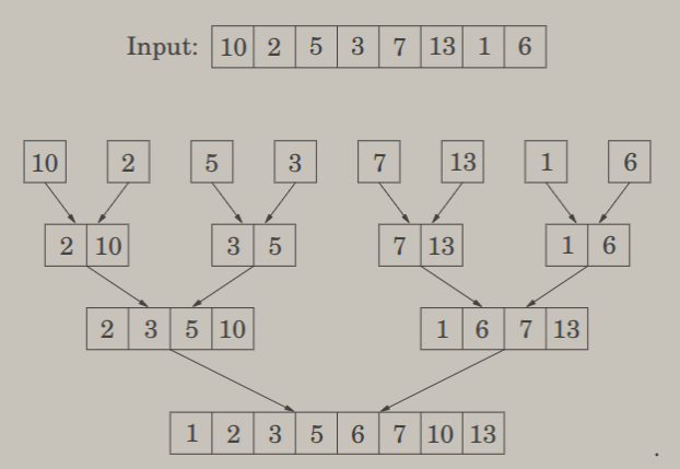
Merging can be done in $O(n)$, the subtree splits in $2$ at every level, and the subproblem size halves between levels. Thus, the recurrence relation is

Which comes out to be $O(n\log n)$.

Mergesort can actually be made iterative by queuing all singleton arrays at the beginning, and at each step removing popping two arrays, merging them, and pushing them into the queue.

Once can actually note that the time complexity of general sorting (not including specialized sorting algorithms like radix sort) is $\Omega(n\log n)$, i.e. lower bound. This is derived by considering the number of comparisons required for sorting an array by creating a binary tree with all possible permutations as the leaves and comparisons as the intermediary (non-root and non-leaf) nodes. Thus, the depth of the tree (number of comparisons required) is at least $\log(n!)$. By Stirling's Formula,

Thus, $\log(n!)\geq n\log n$, and sorting's time complexity is at least $n\log n$. Thus, mergesort is optimal!

2.4 Medians

The naive solution to find a median is sorting. However, this has $O(n\log n)$ time complexity. We can do better!

Randomized

Description

We can use a randomized divide-and-conquer algorithm. It is known as quickselect, and can actually be used for finding the $k$th smallest number, not just the median. It is very similar to quicksort.

$\text{QuickSelect}(S: \text{array},\ k:\text{int})$

1. Randomly pick a pivot point $v$ from the array $S$
2. Split $S$ into three arrays, $S_{\ell},S_{v},S_{r}$ defined as follows:

3. Return one of the following, which may require recursion:

The three arrays $S_{\ell},S_{v},S_{r}$ can be computed from $S$ in $O(n)$ time complexity. And, at each step, the subproblem shrinks to a size of $\mathrm{\mathrm{max}(\lvert S_{\ell} \rvert,\lvert S_{r} \rvert)}$.

Asymptotic Analysis

Since this is a randomized algorithm, its time complexity is dependent on the choice of pivot.

Worst Case

The worst case scenario occurs when our chosen pivot is always the largest or smallest element of the array. This will cause the subproblem to shrink by only one element each time, which results in a time complexity of

However, this is probabilistically impossible.

Best Case

The best case scenario occurs when our chosen pivot is always the median. This results in the recurrence relation

By the Master Theorem, this is just $O(n)$. Again, though, this is extremely unlikely to occur.

Average

Let $v$ be the chosen pivot. Let $v$ be good if it is within the interquartile range (25th to 75th) percentile of the array. Good choices of $v$ guarantee that $\lvert S_{\ell} \rvert,\lvert S_{r} \rvert\leq \frac{3}{4}\lvert S \rvert$. And we expect to pick, on average, $2$ choices of $v$ before getting a good $v$.

Proof
Let $E$ be the expected number of choices before a good $v$. If the current choice is good, we're done. If the current choice is bad, we need to repeat. Thus, $E=1+\frac{1}{2}E$. That is, $E=2$.

Thus, on average, after two split operations, the subproblem will be at most $\frac{3}{4}$ of the original problem size. Therefore, we can write the average recurrence relation

Note that it would be $2O(n)$ since its two split operations, but we ignore constant factors as usual.

Using the Master Theorem, we can conclude that $T(n)=O(n)$. In other words, the algorithm should return the correct answer in linear time complexity, on average.

Deterministic

Description

There also exists a deterministic divide-and-conquer version of $\text{QuickSelect}$ that uses as pivot algorithm known as median of medians. It is parameterized by $x$, the size of each subarray constructed. $x$ must be at least $4$.

$\text{MedianOfMedians}(S:\text{array},\ x:\text{int})$

1. Split the array into contiguous subarrays of size $k$.
2. Find the median of each array by calling the algorithm on each array. (Or, alternatively, using a naive subroutine since $x$ is generally small).
3. Find the median of the medians $m$ by recursively calling the algorithm on the array of medians.
4. The median of medians is used to choose to recurse on at most 70% of the array, with the exact proportion dependent on the value of $k$ in $\text{QuickSelect}$ (assuming $x=5$). See [[#Deterministic#Asymptotic Analysis|below]] for an explanation of how the split works.

Asymptotic Analysis

We will choose $x=5$ for convenience of analysis, and analyze the time complexity of $\text{QuickSelect}$ when using $\text{MedianOfMedians}$ as a pivot selection algorithm.

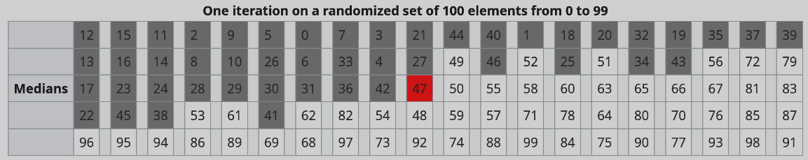First, we will consider how we are able to eliminate 30% of the array. Consider the image above. Here, an array of 100 elements has been divided into 20 subarrays of size 5. The medians are all in row 3, and the median of medians is the element highlighted in red. Everything grayed out is less than the median of medians.

The properties of the median of medians guarantees that everything in the top left corner bounded by the row and column of the median of medians (row 1 to 3, columns 1 to 10). This makes sense because the median of medians is greater than all the median of all subarrays of size 5 before it, and the median of each subarray is greater than the elements above it in the table.

In other words, finding the median of medians allows us to identify with certainty the lower 30% of array elements. A similar thought process follows to identify the upper 30% of array elements.

Therefore, instead of fully partitioning the array based on a pivot, we can use the median of medians as a pivot and subsequently recurse on either the lower or upper of 70% of the array based on $k$. We cannot recurse on the lower/upper 30% of the array because there exist some values not within those regions that are less/greater than the median of medians, respectively.

Thus, the recurrence relation is

The $T(n/5)$ is for finding the median of the medians, the $T\left( \frac{7}{10}n \right)$ is for the next subproblem, and the $O(n)$ is for the partitioning.

To derive the explicit time complexity it helps to draw out the tree for a recurrence relation of the form $T(n)=T(an)+T(bn)$. I'm not dedicated enough to draw a tree, but you'll notice that the total sum of the subproblem sizes at the $k$th level is $(a+b)^{k}n$. Since the combination step (partitioning) is $O(n)$ complexity, the time complexity of the $k$th level is $O((a+b)^{k}n)$. Note that this means the time complexity is simply a geometric series.

Where $k$ here represents the last level. Recall that, in previous proofs, either the first or last term dominates in a finite geometric series. Here, the common ratio depends on $a+b$. For our recurrence relation, $a+b=\frac{1}{5}+\frac{7}{10}=\frac{9}{10}<1$. Therefore, the first term dominates. That is,

2.5 Matrix Multiplication

We will assume we are multiplying 2 $n\times n$ matrices. The naive algorithm for matrix multiplication is $O(n^{3})$, as there are $O(n^{2})$ entries to be computed, and each requires $O(n)$ time.

We can form a naive divide-and-conquer algorithm too, by splitting each matrix into $n/2\times n/2$ blocks, and computing their products before combining. Unfortunately, the recurrence relation is

Which comes out to $O(n^{3})$. However, Volker Strassen came up with a very clever improvement on this divide-and-conquer algorithm. In particular, he figured out how to compute the product of two $n\times n$ matrices $X$ and $Y$ from just seven $n/2\times n/2$ subproblems.

Where

The new recurrence relation is

Applying the Master Theorem gives us $O(n^{\log_{2}7})\approx O(n^{2.81})$.

Aside: Binary Exponentiation

Naive

The naive exponentiation algorithm to calculate $a^{n}$ is to just multiply $a$ with itself times. This has a time complexity of $\Theta(n)$, if you consider multiplication as a constant time operation. However, multiplication is not constant time for binary exponentiation! Consider that the time complexity of multiplication grows with respect to the number of digits of the number (the maximum between the two being multiplied). Let $a$ have $m$ digits. Then $a^{2}$ has about $2m$ digits, $a^{3}$ has about $3m$ digits, ..., and $a^{n}$ has about $nm$ digits. Thus, the number of digits grows with respect to $n$. Therefore, this has time complexity $O(n^{2.59})$ .

Binary

Instead of doing that, we can use the following algorithm.

def exp(a, n):
	if n % 2 == 1: return a * exp(a*a, n>>2)
	else: return exp(a*a, n>>2)

This has $O(\log n)$ time complexity without considering the time complexity of multiplication. Considering the complexity of multiplication, it has time complexity $O(\log n\cdot n^{1.59})$.

Aside: Fibonacci Sequence

Naive

The naive algorithm for the Fibonacci sequence is simply to do a simple recursion.

def fib(n):
	if n == 0: return n
	if n == 1: return n
	return fib(n - 1) + fib(n - 2)

However, this has exponential time complexity. We proceed via induction.

The recurrence relation is $T(n)=T(n-1)+T(n-2)+O(1)$. We seek to prove that the time complexity is $O(2^{n})$.

Base Case: $n=1$
Trivial.

Inductive Hypothesis: $1\leq n\leq k$
Assume the time complexity is $O(2^{n})$ for $1\leq n\leq k$.

Inductive Step: $n=k+1$

Thus, the time complexity is $O(2^{n})$. In fact, we can product an even tighter bound of $O(\phi^{n})$, where $\phi$ is the golden ratio. This can be intuitively explained as follows.

Assume $T(n)=a^{n}$, where $a\in \mathbb{R}^{+}$. Then,

Dynamic Programming

We can definitely compute it faster though! Notice how we are recomputing values we already computed? (In other words, calling Fib with the same argument multiple times). We can instead memoize this, remembering what the output of Fib was for that input.

def fib(n):
	dp = [0 for _ in range(n + 1)]
	dp[1] = 1
	for i in range(2, n + 1):
		dp[i] = dp[i - 1] + dp[i - 2]
	return dp[n]

This allows for linear time complexity... right?

Sorta. If you consider addition to be an $O(1)$ operation, then, yes, this is $O(n)$. Technically, addition is an $O(n)$ operation for the Fibonacci sequence! Let's set some bounds for the Fibonacci sequence.

But also, since $F_{n-2}<F_{n-1}$,

Therefore, $2^{n/2}<F_{n}<2^{n}$. With this, $n$ is a good approximation of the number of digits of $F_{n}$. (Technically, $n/3$, but constant factors don't matter). Therefore, the addition operation actually takes $O(n)$ time complexity for calculating $F_{n}$.

We thus must consider the number of steps for the addition operation at every step of the for loop. The total sum is

Thus, the dynamic programming method actually has a time complexity of $O(n^{2})$.

Binary Matrix Exponentiation

We can note the following formula for calculating the Fibonacci sequence:

Extrapolating, we get

Through matrix diagonalization, we can make the time complexity of binary matrix exponentiation essentially equivalent in time complexity to [[#Binary|binary integer exponentiation]]. Thus, the fastest algorithm is actually $O(\log n\cdot n^{1.59})$.

*Note that taking the limit of this matrix exponentiation produces the golden ratio $\phi$, as confirmed in the previous algebraic derivation of $\phi$.

Aside: Closest Pair

Given a set $P$ of $n$ points in a plane, calculate the Euclidean distance between the closest pair of points.

Naive

There is clearly an $O(n^{2})$ algorithm that checks the distance between every pair of points, and finds the minimum.

Divide and Conquer

Algorithm

Choose a pivot point $(x,y)$ in the middle of the points in terms of $x$-coordinate. Divide the graph into two sets $L$ and $R$, corresponding to points left and right of the pivot, respectively. Then, calculate the closest pair distance in $L$ and the closest pair distance in $R$ by recursing the algorithm on these subproblems. Let $d_{L},d_{R}$ denote these distances. Let $d=\mathrm{min}(d_{L},d_{R})$. We can prove some properties for this problem.

Property 1: If $p \in L$, $q\in R$, and $\Delta(p,\ q)$ (distance between $p$ and $q$) is less than $d$, then $\lvert p.x-\text{pivot}_{x} \rvert<d$ and $\lvert q.x-\text{pivot}_{x} \rvert < d$.

Proof: We proceed via proof by contraposition. Let $p$ lie outside the region of the plane where $\text{pivot}_{x}-d<x<\text{pivot}_{x}+d$. Since $q\in R$, $\Delta(p.x,\ q.x)>\Delta(p,\ (\text{pivot}_{x},\ p.y))$ Then, it is guaranteed that $\lvert p.x-\text{pivot}_{x} \rvert\geq d\implies \Delta(p,\ q)\geq d$.

$\square$

Property 2: Any tile $T$ that is $\frac{d}{2}\times \frac{d}{2}$ in size that is entirely contained in $L$ or $R$ can have at most one point.

Proof: We proceed via contradiction. Assume $\exists p,q\in S$ and $p,q$ are contained in $T$. Then, $\Delta(p,q)\leq \sqrt{ \left( \frac{d}{2} \right)^{2}+\left( \frac{d}{2} \right)^{2} }=\frac{d}{\sqrt{ 2 }}<d$. That is, this pair of points would have formed the closest pair in $L$ or $R$, which is a contradiction.

$\square$

Property 3: Let $p$ lie inside the region of the plane where $\text{pivot}_{x}-d<x<\text{pivot}_{x}+d$. Then, there are at most $7$ points in $P$ within the same region such that $p.y\leq q.y$ and $\Delta(p,\ q)$ could be less than $d$.

Proof: Consider the $2d\times d$ region within the aforementioned $\text{pivot}_{x}-d<x<\text{pivot}_{x}+d$ region where $p$ lies in the vertical bottom of the $2d\times d$ region. Subdivide the $2d\times d$ region into $8$ $\frac{d}{2}\times \frac{d}{2}$ squares, and arbitrarily assign $p$ to one of the squares it borders. Consider that any point $q$ above this $2d\times d$ region certainly has $\Delta(p,\ q)\geq\Delta(p.y,\ q.y)\geq d$. Therefore, $q$ must exist within one of the other $7$ squares $\implies$ there are at most $7$ points in $P$ within the same region such that the statement is true.

$\square$

We can now describe the algorithm.

1. First, we preprocess the set of points $P$, producing a list $P_{x}$, the set of points sorted by $x$, and $P_{y}$, the analogue for $y$.
2. We define a function $\text{Closest}(P_{x},P_{y})$
   1. Let $n=\lvert P_{x} \rvert$. If $n\leq3$, just brute force.
   2. Choose the middle pivot point, "middle" in terms of $x$. Partition $P_{x}$ into $L_{x}$ and $R_{x}$ in $O(1)$ time. Partition $P_{y}$ into $L_{y}$ and $R_{y}$ in $O(n)$ time. These lists should remain sorted according to their subscript.
   3. Recurse on the subproblems. That is, $d_{L}=\text{Closest}(L_{x},L_{y})$ and $d_{R}=\text{Closest}(R_{x},R_{y})$. Then, $d=\mathrm{min}(d_{L},d_{R})$,
   4. Define the middle $2d\times d$ region (strip) and conquer. We write the pseudocode here:

      # construct strip, sorted by y
      strip = []
      for p in Py:
          if abs(p.x - pivot.x) < d:
       	   strip.append(p)
      
       # process closest pair candidates
       k = len(strip)
       for i in range(k):
       	for j in range(i + 1, k): # this will run at most 7 times
       		if strip[j][1] - strip[i][1] >= d:
       			break
       		d = min(d, distance(strip[i], strip[j]))
      

Time Complexity Analysis

Preprocessing takes $O(n\log n)$ time. Partitioning takes $O(n)$ time. Recursing on the subproblems takes $2T(n/2)$ time. Processing the strip takes $O(n)$ time, with a small constant factor. The recurrence relation is thus

By the Master Theorem, $T(n)=O(n\log n)$. Since preprocessing also has $O(n\log n)$ time complexity, the overall algorithm has $O(n\log n)$ time complexity!

$\square$