Lecture 20: Reinforcement Learning Theory

Why study RL theory?

First, there are some interesting questions asked in RL theory.

If I use algorithm $\mathcal{A}$ $A$ with $N$ $N$ samples for $k$ $k$ iterations, what is the worst case performance (under some set of assumptions)?
- For instance, determining the number of iterations $k$ of $Q$ -learning to produce $\lVert \hat{Q}_{k}-Q^{*} \rVert\leq\epsilon$ with probability $\geq 1- \delta$ if $N\geq f(\epsilon,\delta)$ .
- Or, determining the number of iterations $k$ of $Q$ -learning such that $\lVert Q^{\pi_{k}}-Q^{*} \rVert\leq\epsilon$ .
For some exploration algorithm $\mathcal{A}$ , how high, in the worst-case, is the regret?
And many others!

In analyzing RL theory, it's also necessary to make some strong assumptions to achieve any interesting results, while not deviating too far from reality. For...

...exploration: how likely are we to find (potentially sparse) rewards? In the worst case, it's extremely hard; thus, there are typically some assumptions made to produce interesting bounds.
...learning: how many samples do we need to effectively learn a model/value function? Often, a "generative model" assumption is made that assumes we can sample from $p(s'\mid s,a)$ for any $(s,a)$ (assumes exploration is not too hard). Alternatively, an "oracle exploration" assumption assumes sampling from $p(s'\mid s,a)$ for each $(s,a)$ up to $N$ times.

The point of this is not to prove that an algorithm works perfectly every time (in fact, in deep RL, typically not even convergence is guaranteed). However, it does yield interesting conclusions on the effect of problem parameters/hyperparameters on error—RL theory produces qualitative conclusions about various factors under strong assumptions that are reasonable enough such that they may guide decisions in real RL problems..

Some Useful Identities

\begin{align*} Q^{\pi}(s,a) &= r(s,a)+\gamma \mathbb{E}_{s'\sim p(s'\mid s,a)}[V^{\pi}(s')]=r(s,a)+\gamma \sum_{s'}p(s'\mid s,a)V^{\pi}(s') \implies \\ Q^{\pi} &= r + \gamma PV^{\pi} \\ \\ p^{\pi}(s',a'\mid s,a) &= \pi(a'\mid s')p(s'\mid s,a) \implies \\ Q^{\pi} &= r + \gamma P^{\pi}Q^{\pi} \\ \\ Q^{\pi}-\gamma P^{\pi}Q^{\pi} &= r \\ (\mathbf{I}-\gamma P^{\pi})Q^{\pi} &= r \\ Q^{\pi} &= (I-\gamma P^{\pi})^{-1}r \end{align*}

Note that $r$ is a vector, and $Q^{\pi},P,P^{\pi},V^{\pi}$ are all matrices.

That final equation actually gives us a method of recovering the $Q$ -function, but is impractical not just for the typically high dimensionality of the state and action spaces but because we typically do not assume knowledge of $P^{\pi}$ (involves state transition probabilities). Notably, though, that last equation tells us that policy evaluation is essentially just a linear operation.

Now, say $r\approx1$ . From this, we can note that $\sum_{t=0}^{\infty}\gamma^{t}r\approx \sum_{t=0}^{\infty}\gamma^{t}=\frac{1}{1-\gamma}$ . Thus, the total reward of a trajectory is approximately $\frac{1}{1-\gamma}$ , and thus our $Q$ -function matrix $Q^{\pi}$ has elements that are roughly $\frac{1}{1-\gamma}$ in magnitude. Alternatively, for a finite horizon problem (and no discounting), we have that the total reward of a trajectory is approximately $\sum_{t=1}^{H}r\approx H$ , and our $Q$ -function matrix $Q^{\pi}$ would have elements that are roughly $H$ in magnitude. Therefore, for infinite horizon tasks with discounting, we can roughly term $\frac{1}{1-\gamma}$ as a "finite horizon" for the problem.

Convergence of Value Iteration

In linear algebra notation, value iteration is $V\leftarrow \max_{a}[r+\gamma PV]$ . Let's define an operator $T$ such that

TV=\max _{a}[r+\gamma PV]

this is known as the Bellman optimality operator. Also, let us note the following useful inequality

\lvert \max _{x}f(x)-\max _{x}g(x) \rvert \leq \max _{x}\lvert f(x)-g(x) \rvert

Consider, now, two value functions $V(s)$ and $U(s)$ . We'll apply the Bellman optimality operator to both, and consider the difference.

\begin{align*} \lvert TV(s)-TU(s) \rvert &= \left\lvert \max _{a}\left[ r(s,a)+\gamma \sum_{s'}p(s'\mid s,a)V(s') \right]-\max _{a}\left[ r(s,a)+\gamma \sum_{s'}p(s'\mid s,a)U(s') \right] \right\rvert \\ &\leq \max _{a}\left\lvert \sum_{s'}p(s'\mid s,a)(V(s')-U(s')) \right\rvert \\ &\leq \gamma\max _{s'}\lvert V(s')-U(s') \rvert \\ &= \gamma \lVert V-U \rVert _{\infty} \end{align*}

Thus, applying $T$ to any two value functions $V$ and $U$ will "bring them closer" w.r.t. to the infinity norm.

Also, we will note that $TV^{*}=V^{*}$ , or that the optimal value function does not change by application of the Bellman optimality operator. We will not prove this fact for brevity.

Therefore,

\begin{align*} \lVert TV-V^{*} \rVert _{\infty} &= \lVert TV-TV^{*} \rVert _{\infty} \leq \lVert V-V^{*} \rVert _{\infty} \\ \lVert T^{k}V-V^{*} \rVert _{\infty} &\leq \gamma^{k}\lVert V-V^{*} \rVert _{\infty} \\ \lim_{ k \to \infty } \lVert T^{k}V-V^{*} \rVert _{\infty} &= 0 \end{align*}

And thus value iteration converges!

Sample Complexity without Exploration

First, let's define our algorithm and assumptions. We will assume "oracle exploration," i.e. we can sample $s'\sim p(s'\mid s,a)$ for each $(s,a)$ up to $N$ times. Our algorithm is a simple "model based" algorithm.

$\hat{p}(s'\mid s,a)=\frac{\#(s,a,s')}{N}$ .
Given $\pi$ , use $\hat{p}$ to estimate $\hat{Q}^{\pi}$ .

Then, we'd like to answer the following questions.

How close is $\hat{Q}^{\pi}$ to $Q^{\pi}$ ?
How close is $\hat{Q}^{*}$ to $Q^{*}$ if we learn it using $\hat{p}$ ?
How close is the final policy $Q^{\hat{\pi}^{*}}$ to $Q^{*}$ ?

We'll first address question 1, where we define $(\epsilon,\delta)$ -closeness as $\lVert Q^{\pi}(s,a)-\hat{Q}^{\pi}(s,a) \rVert_{\infty}\leq\epsilon$ with probability at least $1-\delta$ if $N\geq f(\epsilon,\delta)$ . Note that we use $\lVert \cdot \rVert_{\infty}$ because it provides worst-case performance bounds.

Concentration Inequalities

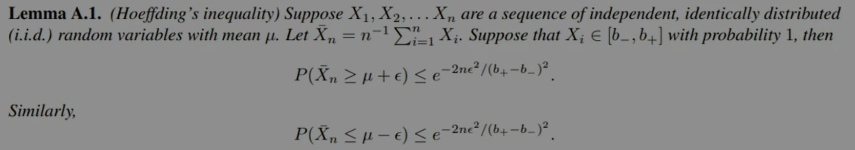
Now, relating samples to errors is highly nontrivial. We will need a concentration inequality; Perhaps the simplest such inequality is Hoeffding's inequality.

Intuitively, the interpretation is that if we estimate $\mu$ with $n$ samples the probability we're off by more than $\epsilon$ is at most $2e^{ -2n\epsilon^{2}/(b_{+}-b_{-})^{2} }$ .

Equivalently, if we want this probability bound to be $\delta$ , we can show that we require

\frac{b_{+}-b_{-}}{\sqrt{ 2n }}\sqrt{ \log \frac{2}{\delta} } \geq \epsilon

Importantly, $\epsilon \propto \frac{1}{\sqrt{ n }}$ .

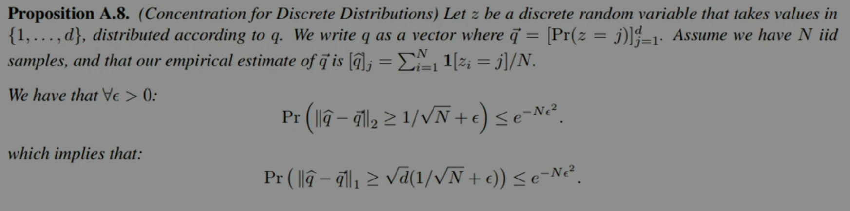
However, we are estimating sample probabilities, not sample averages. For that, we need a different concentration inequality.

From this, we derive

\delta \leq \frac{1}{\sqrt{ N }}\sqrt{ \log \frac{1}{\delta} }

and we may apply this to our problem and write

\begin{align*} \lVert \hat{p}(s'\mid s,a)-p(s'\mid s,a) \rVert_{1} &\leq \sqrt{ \lvert S \rvert }\left( \frac{1}{\sqrt{ N }}+\epsilon \right),\text{ with probability } 1-\delta \\ &= \sqrt{ \frac{\lvert S \rvert }{N} } + \sqrt{ \frac{\lvert S \rvert \log \frac{1}{\delta}}{N} } \\ &\leq c\sqrt{ \frac{\lvert S \rvert \log \frac{1}{\delta}}{N} } \end{align*}

for some constant $c$ .

Useful Lemmas

We'd like to now relate the error of $\hat{p}$ to the error of $\hat{Q}^{\pi}$ . We can note that

\begin{align*} Q^{\pi} &= r+\gamma PV^{\pi} \\ V^{\pi} &= \Pi Q^{\pi} \\ P^{\pi} &= P\Pi \end{align*}

Note that $\Pi$ represents the matrix of $\pi(a\mid s)$ for all $(s,a)$ , and $P$ represents the matrix of $p(s'\mid s,a)$ for all $(s,a,s')$ . These directly imply that

\begin{align*} Q^{\pi} &= r+\gamma P^{\pi}Q^{\pi} \\ Q^{\pi} &= (I-\gamma P^{\pi})^{-1}r \end{align*}

Comparing this with the previous equation derived for $\hat{Q}^{\pi}$ , we note the similarity

\begin{align*} Q^{\pi} &= (I-\gamma P^{\pi})^{-1}r \\ \hat{Q}^{\pi} &= (I-\gamma \hat{P}^{\pi})^{-1}r \end{align*}

Then, we claim the following simulation lemma is true.

Q^{\pi}-\hat{Q}^{\pi} = \gamma(I-\gamma \hat{P}^{\pi})^{-1}(P-\hat{P})V^{\pi}

Proof.

\begin{align*} Q^{\pi} - \hat{Q}^{\pi} &= Q^{\pi}-(I-\gamma \hat{P}^{\pi})^{-1}r \\ &= (I-\gamma \hat{P}^{\pi})^{-1}(I-\gamma \hat{P}^{\pi})Q^{\pi}-(I-\gamma \hat{P}^{\pi})^{-1}r \\ &= (I-\gamma \hat{P}^{\pi})^{-1}(I-\gamma \hat{P}^{\pi})Q^{\pi}-(I-\gamma \hat{P}^{\pi})^{-1}(I-\gamma P^{\pi})Q^{\pi} \\ &= (I-\gamma \hat{P}^{\pi})^{-1}((I-\gamma \hat{P}^{\pi})Q^{\pi}-(I-\gamma P^{\pi})Q^{\pi}) \\ &= \gamma(I-\gamma \hat{P}^{\pi})^{-1}(P^{\pi}-\hat{P}^{\pi})Q^{\pi} \\ &= \gamma(I-\gamma \hat{P}^{\pi})^{-1}(P\Pi-\hat{P}\Pi)Q^{\pi} \\ &= \gamma(I-\gamma \hat{P}^{\pi})^{-1}(P-\hat{P})\Pi Q^{\pi} \\ &= \gamma(I-\gamma \hat{P}^{\pi})^{-1}(P-\hat{P})V^{\pi} \\ \end{align*}

Another useful lemma is that, for some $P^{\pi}$ and any vector $v\in \mathbb{R}^{\lvert S \rvert \lvert A \rvert}$ , we have that

\lVert (I-\gamma P^{\pi})^{-1}v \rVert _{\infty} \leq \lVert v \rVert _{\infty}/(1-\gamma)

this is basically just a formalization of an obvious fact using the geometric series application with $\gamma$ previously. It's really just stating that, in policy evaluation, the maximum $Q$ -function value is bounded by the maximum reward seen across all time steps multiplied by the effective horizon $\frac{1}{1-\gamma}$ .

Proof.
Let $w=(I-\gamma P^{\pi})^{-1}v$ .

\begin{align*} \lVert v \rVert _{\infty} &= \lVert (I-\gamma P^{\pi})w \rVert _{\infty} \\ &\geq \lVert w \rVert _{\infty}-\gamma \lVert P^{\pi}w \rVert _{\infty} && \text{(Triangle Inequality)} \\ &\geq \lVert w \rVert _{\infty} - \gamma \lVert w \rVert _{\infty} && (\lVert P^{\pi} \rVert _{\infty}\leq 1) \\ &= (1-\gamma)\lVert w \rVert _{\infty} \implies \\ \lVert v \rVert _{\infty} /(1-\gamma) &\geq \lVert (I-\gamma P^{\pi})^{-1}v \rVert_{\infty} \end{align*}

Putting it Together

Now, let's apply both lemmas and finish off the error bound.

\begin{align*} Q^{\pi}-\hat{Q}^{\pi} &= \gamma(I-\gamma \hat{P}^{\pi})(P-\hat{P})V^{\pi} && \text{(Simulation Lemma)} \\ \lVert Q^{\pi}-\hat{Q}^{\pi} \rVert _{\infty} &= \lVert \gamma(I-\gamma \hat{P}^{\pi})(P-\hat{P})V^{\pi} \rVert_{\infty} \\ &\leq \frac{\gamma}{1-\gamma} \lVert (P-\hat{P})V^{\pi} \rVert _{\infty} && \text{Lemma 2} \\ &\leq \frac{\gamma}{1-\gamma}(\max _{s,a}\lVert p(\cdot \mid s,a) -\hat{p}(\cdot \mid s,a) \rVert_{1})\lVert V^{\pi} \rVert _{\infty} \\ \end{align*}

Note that $\lVert V^{\pi} \rVert_{\infty}\leq \frac{1}{1-\gamma}R_{\text{max}}$ because of the same geometric series trick, and we can actually assume WLOG $R_{\text{max}}=1$ because, if they aren't, we can simply rescale the rewards appropriately (if we multiply the rewards by any constant, the optimal policy doesn't change). Thus, $\lVert V^{\pi} \rVert_{\infty} \leq \frac{1}{1-\gamma}$ . Thus,

\begin{align*} \lVert Q^{\pi}-\hat{Q}^{\pi} \rVert _{\infty} &\leq \frac{\gamma}{(1-\gamma)^{2}}(\max _{s,a}\lVert p(\cdot \mid s,a) -\hat{p}(\cdot \mid s,a) \rVert_{1}) \end{align*}

Now recall the concentration inequality.

\lVert \hat{p}(s'\mid s,a)-p(s'\mid s,a) \rVert \leq c\sqrt{ \frac{\lvert S \rvert \log \frac{1}{\delta}}{N} }

Which allows us to conclude that our error bound is

\lVert Q^{\pi}-\hat{Q}^{\pi} \rVert _{\infty} \leq \frac{\gamma}{(1-\gamma)^{2}}c_{2}\sqrt{ \frac{\lvert S \rvert \log \frac{1}{\delta}}{N} }=\epsilon

Note that $c_{2}$ exists because there is some constant factor involved when substituting for the lemma.

Interpretation

So, what can we take away from our error bound $\epsilon$ ?

First, the error grows quadratically in the horizon and each backup "accumulates" error.

\epsilon\propto \frac{1}{(1-\gamma)^{2}}

Second, more samples translates to lower error.

\epsilon\propto \sqrt{ \frac{1}{N} }

Implications about Other Questions

What about the other questions we asked previously?

Let's first consider the second, i.e. bounding $\lVert Q^{*}-\hat{Q}^{*} \rVert$ . Note the following lemma

\lvert \sup_{x}f(x)-\sup_{x}g(x) \rvert \leq \sup_{x}\lvert f(x)-g(x) \rvert

(This is essentially the same as the previous inequality just with $\sup$ , supremum, instead of $\max$ ).

Then,

\begin{align*} \lVert Q^{*}-\hat{Q}^{*} \rVert _{\infty} &= \lVert \sup_{\pi}Q^{\pi}-\sup_{\pi}\hat{Q}^{\pi} \rVert _{\infty} \leq \sup_{\pi}\lVert Q^{\pi}-\hat{Q}^{\pi} \rVert _{\infty} \leq \epsilon \end{align*}

Now, let's consider the third, i.e. bounding $\lVert Q^{*}-Q^{\hat{\pi}^{*}} \rVert_{\infty}$ .

\begin{align*} \lVert Q^{*}-Q^{\hat{\pi}^{*}} \rVert _{\infty} &= \lVert Q^{*}-\hat{Q}^{\hat{\pi}^{*}}+\hat{Q}^{\hat{\pi}^{*}}-Q^{\hat{\pi}^{*}} \rVert _{\infty} \\ &\leq \lVert Q^{*}-\hat{Q}^{\hat{\pi}^{*}} \rVert _{\infty} + \lVert Q^{\hat{\pi}^{*}}-\hat{Q}^{\hat{\pi}^{*}} \rVert_{\infty} \\ \end{align*}

We note that $\hat{Q}^{\hat{\pi}^{*}}$ is essentially just $\hat{Q}^{*}$ , and so the first term is bounded by $\epsilon$ according to our second derived bound, $\lVert Q^{*}-\hat{Q}^{*} \rVert_{\infty}\leq\epsilon$ . Meanwhile, the second infinity norm is bounded by $\epsilon$ according to our first derived bound, $\lVert Q^{\pi}-\hat{Q}^{\pi} \rVert\leq\epsilon$ , where $\pi=\hat{\pi}^{*}$ here. Thus,

\lVert Q^{*}-Q^{\hat{\pi}^{*}} \rVert _{\infty} \leq 2\epsilon

Analysis of Model-Free RL

We'll now analyze fitted $Q$ -iteration.

First, let $T$ be the Bellman operator such that

TQ = r+\gamma P\max _{a}Q

Then, exact fitted $Q$ -iteration may be defined as $Q_{k+1}\leftarrow TQ_{k}$ . For approximate fitted $Q$ -iteration that uses samples, it changes slightly to be $\hat{Q}_{k+1}\leftarrow \arg\min_{Q}\lVert \hat{Q}-\hat{T}\hat{Q}_{k} \rVert$ . $\hat{T}$ is the Bellman operator, except it accounts for sampling by considering the effective frequency of observations of each $s'$ . In particular, we define $\hat{T}$ as

\hat{T}Q = \hat{r}+\gamma \hat{P}\max _{a}Q

where

\begin{align*} \hat{r} &= \frac{1}{N(s,a)}\sum_{i}\delta((s_{i},a_{i})=(s,a))r_{i} \\ \hat{p}(s'\mid s,a) &= \frac{N(s,a,s')}{N(s,a)} \end{align*}

However, our update rule now involves a norm—what norm should we use? Unfortunately, the algorithm won't actually converge if $\lVert \cdot \rVert_{2}$ is used; therefore, we will assume $\lVert \cdot \rVert_{\infty}$ . Notably, no such learning algorithm exists that may train with the infinity norm, and mean squared error is of course used in practice. Some interesting properties of the MSE-based learning algorithm are provable; however, they are much more difficult. Thus, we proceed with a theoretical learning algorithm that works with the infinity norm.

Now, we'd like to answer the following question: as $k\to \infty$ , $\hat{Q}_{k}\to\; ?$ or $\lim_{ k \to \infty }\lVert \hat{Q}_{k}-Q^{*} \rVert_{\infty}\leq\; ?$ . Where does our error come from though? For approximate fitted $Q$ -iteration, from sampling error, $T\neq \hat{T}$ , and approximation error, $\hat{Q}_{k+1}\neq \hat{T}\hat{Q}_{k}$ .

Sampling Error

Let's first understand the effect of sampling error.

\begin{align*} \lvert \hat{T}Q(s,a)-TQ(s,a) \rvert &= \lvert \hat{r}(s,a)-r(s,a) +\gamma(\mathbb{E}_{\hat{p}(s'\mid s,a)}[\max _{a'}Q(s',a')]-\mathbb{E}_{p(s'\mid s,a)}[\max _{a'}Q(s',a')]) \rvert \\ &\leq [\hat{r}(s,a)-r(s,a)]+\gamma \left\lvert \sum_{s'}(\hat{p}(s'\mid s,a)-p(s'\mid s,a))\max _{a'}Q(s',a') \right\rvert \end{align*}

Where the inequality applied is triangle inequality. For the first term, the estimation of a continuous random variable, we can use Hoeffding's inequality.

\lvert \hat{r}(s,a)-r(s,a) \rvert \leq 2R_{\text{max}}\sqrt{ \frac{\log \frac{1}{\delta}}{2N} }

Meanwhile, for the second term, we can use the other concentration inequality

\begin{align*} \left\lvert \sum_{s'}(\hat{p}(s'\mid s,a)-p(s'\mid s,a))\max _{a'}Q(s',a') \right\rvert &\leq \sum_{s'}\lvert \hat{p}(s'\mid s,a)-p(s'\mid s,a) \rvert \max _{s',a'}Q(s',a') \\ &= \lVert \hat{p}(\cdot \mid s,a)-p(\cdot \mid s,a) \rVert_{1}\lVert Q \rVert _{\infty} \\ &\leq c\lVert Q \rVert _{\infty}\sqrt{ \frac{\log \frac{1}{\delta}}{N} } \end{align*}

Thus, we can bound our error as

\begin{align*} \lvert \hat{T}Q(s,a)-TQ(s,a) \rvert &\leq 2R_{\text{max}} \sqrt{ \frac{\log \frac{1}{\delta}}{2N} } + c\lVert Q \rVert _{\infty}\sqrt{ \frac{\log \frac{1}{\delta}}{N} } \end{align*}

Using the union bound, we can derive

\begin{align*} \lvert \hat{T}Q(s,a)-TQ(s,a) \rvert &\leq 2R_{\text{max}}c_{1} \sqrt{ \frac{\log \frac{\lvert S \rvert \lvert A \rvert }{\delta}}{2N} } + c_{2}\lVert Q \rVert _{\infty}\sqrt{ \frac{\log \frac{\lvert S \rvert }{\delta}}{N} } \end{align*}

Approximation Error

We'll first analyze the exact backup operator. We will assume $\lVert \hat{Q}_{k+1}-T\hat{Q}_{k} \rVert_{\infty}\leq\epsilon_{k}$ for some $\epsilon_{k}$ . Note that this is a pretty strong assumption!

\begin{align*} \lVert \hat{Q}_{k}-Q^{*} \rVert _{\infty} &= \lVert \hat{Q}_{k}-T\hat{Q}_{k-1} +T\hat{Q}_{k-1}+Q^{*} \rVert \\ &= \lVert (\hat{Q}_{k}-T\hat{Q}_{k-1})+(T\hat{Q}_{k-1}-TQ^{*}) \rVert_{\infty} \\ &\leq \lVert \hat{Q}_{k}-T\hat{Q}_{k-1} \rVert_{\infty} +\lVert T\hat{Q}_{k-1}-TQ^{*} \rVert_{\infty} \\ &\leq \epsilon_{k-1}+\lVert T\hat{Q}_{k-1}-TQ^{*} \rVert _{\infty} \\ &\leq \epsilon_{k-1} + \gamma\lVert \hat{Q}_{k-1}-Q^{*} \rVert _{\infty} \end{align*}

Recall the substitution of $Q^{*}$ with $TQ^{*}$ in step 2 is possible because $Q^{*}$ is a fixed point of the operator $T$ . The last step leverages the fact that $T$ is a $\gamma$ -contraction. We can recurse through this last inequality to produce

\begin{align*} \lVert \hat{Q}_{k}-Q^{*} \rVert _{\infty} &\leq \sum_{i=0}^{k-1} \gamma^{i}\epsilon_{k-i-1}+\gamma^{k}\lVert \hat{Q}_{0}-Q^{*} \rVert _{\infty} \\ \lim_{ k \to \infty } \lVert \hat{Q}_{k}-Q^{*} \rVert _{\infty} &\leq \sum_{i=0}^{k-1} \gamma^{i}\max _{k}\epsilon_{k} \\ &= \frac{1}{1-\gamma}\lVert \epsilon \rVert _{\infty} \\ &= \frac{1}{1-\gamma}\max _{k} \lVert \hat{Q}_{k}-T\hat{Q}_{k-1} \rVert _{\infty} \end{align*}

In other words, the approximation error scales with horizon.

Putting it Together

Let's now combine our bounds on the approximation error and sampling error to produce a bound on total error.

\begin{align*} \lVert \hat{Q}_{k}-T\hat{Q}_{k-1} \rVert &= \lVert \hat{Q}_{k}-\hat{T}\hat{Q}_{k-1}+\hat{T}\hat{Q}_{k-1}-T\hat{Q}_{k-1} \rVert _{\infty} \\ &\leq \underbrace{ \lVert \hat{Q}_{k}-\hat{T}\hat{Q}_{k-1} \rVert _{\infty} }_{ \text{approximation error} }+\underbrace{ \lVert \hat{T}\hat{Q}_{k-1}-T\hat{Q}_{k-1} \rVert _{\infty} }_{ \text{sampling error} } \\ \end{align*}

Here are the bounds again, for convenience.

\begin{align*} \lvert \hat{T}Q(s,a)-TQ(s,a) \rvert &\leq 2R_{\text{max}}c_{1} \sqrt{ \frac{\log \frac{\lvert S \rvert \lvert A \rvert }{\delta}}{2N} } + c_{2}\lVert Q \rVert _{\infty}\sqrt{ \frac{\log \frac{\lvert S \rvert }{\delta}}{N} } \\ \lim_{ k \to \infty } \lVert \hat{Q}_{k}-Q^{*} \rVert_{\infty} &\leq \frac{1}{1-\gamma}\max _{k} \lVert \hat{Q}_{k}-T\hat{Q}_{k-1} \rVert _{\infty} \end{align*}

Notably, the $\lVert Q \rVert_{\infty}$ in the sampling error bound is in $O\left( R_{\text{max}} \frac{1}{1-\gamma} \right)$ . (Recall from previously that the entries of the $Q$ -function matrix are approximately the size of the horizon, assuming $r\approx1$ ). Meanwhile, there exists a $\frac{1}{1-\gamma}$ scalar for the approximation error bound. Thus, error compounds with quadratically with the horizon, since the error for each step $\lVert \hat{Q}_{k}-T\hat{Q}_{k-1} \rVert$ scales with the horizon and there are $H$ steps for a horizon $H$ .