Lecture 3

Solution 2: Better Models, Less Mistakes

Why might a model fail to fit to the expert (training data)? The human expert may exhibit...

• Non-Markovian behavior
• Multimodal behavior

Non-Markovian Behavior

Instead of $\pi_{\theta}(\mathbf{a}_{t}\mid \mathbf{o}_{t})$, a human's policy resembles something more like $\pi_{\theta}(\mathbf{a}_{t}\mid \mathbf{o}_{1},\dots,\mathbf{o}_{t})$, in which the current behavior depends on all past observations, not just the current observation. This sort of knowledge can be encoded by using some sort of sequence model, e.g. transformer, to process each observation "frame" in history.

However, including history can degrade model performance. Why?

• Access to more (unnecessary) information can cause mistakes.
• It may induce overfitting as the model must naturally be larger and have more capacity.
• It can increase the chance of distributional shift, as even one small deviation remains in the history forever, and therefore contributes to the shift from then on.

Causal confusion is a particularly notable consequence of an excess of information. In essence, a model's action $A$ causes an event $B$, which results in $A$ and $B$ showing up together very frequently. As the model makes associations, not causal relationships, the occurrence of $B$ can actually influence the model into doing $A$. This phenomenon is known as spurious correlation.

Multimodal Behavior

Multimodal behavior describes environments where there exist states for which there are multiple reasonable actions. This becomes an issue with continuous actions, in which a unimodal distribution (e.g. Gaussian) would essentially average the reasonable actions together to produce an action that may not be reasonable at all! There are a couple solutions to this.

• Discretize the continuous action space $\to$ softmax correctly identifies all reasonable actions
• Use more expressive continuous distributions $\to$ multimodal distributions that capture all reasonable actions

Discretization

Can we always just naively discretize continuous action spaces? No, because the number of discrete "bins" is exponential in the dimensionality of the action space. For low-dimensional action spaces, however, this is a great solution.

One may suggest discretizing one dimension at a time to avoid the exponential explosion; however, this is not necessarily effective because it suggests choosing along each dimensions independently when, in fact, the dimensions may covary with each other.

Autoregressive discretization provides a computationally efficient (linear, not exponential) solution for high-dimensional action spaces. In essence, this discretizes one dimension at a time, but in sequence, rather than independently. In essence, the sequence model (e.g. transformer), when predicting dimension $i$ of the action space, is fed the original input (state/observations) and the previously predicted dimensions, i.e. dimensions $0,\dots,i-1$. In short, the dimensions are discretized one a time and then decoded autoregressively (hence the nomenclature).

This is valid by the Chain Rule of Probability. If we denote dimension $i$ of action $\mathbf{a}_{t}$ as $a_{t,i}$, then

In other words, this is equivalent to predicting all dimensions of the action at once based on the state while still providing an efficient method of discretization.

Expressive Continuous Distributions

Generally speaking, it's hard to model multimodal distributions. Instead, we can include an additional input that "decides" the mode that the model chooses; this additional input can simply be some random noise.

The main challenge with this method, however, is that we must train the model to actually use the random noise to decide the mode—otherwise, of course, the noise is useless. There are several different solutions for this.

• Variational autoencoders
• Normalizing flows
• Diffusion/flow matching

Diffusion/Flow Matching

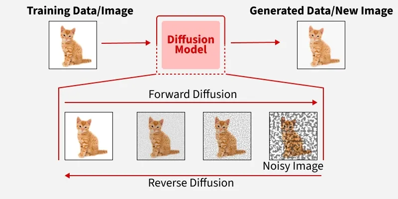
Diffusion is the most popular approach for generating high dimensional, continuous data. The key principle underlying diffusion is that turning random noise into a specific image (e.g. image of a dog) is hard, but turning an image of a dog into random noise is easy (just add more noise). So, to train a model to generate images of dogs, we take real images of dogs, iteratively add noise, and then train the model to simply go the other way!

Source: GeeksforGeeks

Flow matching is the modern version of diffusion, with essentially the same intuition, except it's easier to implement. In essence, we want to train a model to start with a noise distribution, e.g. Gaussian, and transform samples from it into a desired data distribution. It relies on the same idea of starting with real data samples and adding noise, and simply training the model to reverse this process. Formally, flow matching learns a vector field $v(\mathbf{x}_{t},t)$ that allows "sampling from" (modeling) $p(\mathbf{x})$ by sampling $\mathbf{x}_{0}\sim p_{0}(\mathbf{x}_{0})$ (noise distribution) and integrating the vector field to produce $\mathbf{x}_{1}=\mathbf{x}_{0}+\int_{0}^{1} v(\mathbf{x}_{t},t) \, \mathrm{d}t$. In practice, this integration is discretized as Euler integration. Below is a demonstration of flow matching in action.

Source

But how do we train flow matching?

1. Sample $\mathbf{x}_{0}\sim \mathcal{N}(0,\mathbf{I})$ (i.e. Gaussian noise distribution)
2. Sample $\mathbf{x}_{1}\in \mathcal{D}$ where $\mathcal{D}=\{ \mathbf{x}^{(i)} \}_{i=1}^{N}$ (data distribution)
3. Sample $t\sim p(t)$ where $p(t)$ is defined only over $[0,1]$ (e.g. $p(t)=\mathcal{U}(0,1)$), as this is the selection of the "time step" $t$ of the vector field in-between $t=0$, the noise distribution, and $t=1$, the data distribution. See the below diagram for clarification.
4. Compute $\mathbf{x}_{t}=t\mathbf{x}_{1}+(1-t)\mathbf{x}_{0}$ (i.e. just draw a line)
5. Update $v$ with $\nabla \lVert v(\mathbf{x}_{t},t)-(\mathbf{x}_{1}-\mathbf{x}_{0}) \rVert^{2}$, or update the velocity (that point in the vector field) to point more towards $\mathbf{x}_{1}$ (i.e. intended velocity is the slope of the line $(\mathbf{x}_{1}-\mathbf{x}_{0})$)

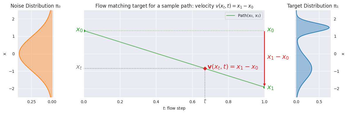
The point of this with regards to fixing the averaging problem is that the vector field produced by flow matching will eventually diverge to produce one of the reasonable actions. In earlier "time" steps ($t$ closer to $0$), the vector field appears more averaged across reasonable actions. When $t$ is closer to $1$, the vector field starts to diverge. In essence, the supervision of many linear vector fields produces an overall vector field that effectively maps the noise distribution to the target distribution, effectively representing multimodality.

In RL, flow matching is applied as follows.

1. Construct minibatch. For each element in batch $j$,
   1. Sample $(\mathbf{o}_{t}^{(j)},\mathbf{a}_{t}^{(j)})$ from dataset (data distribution)
   2. Sample $\mathbf{a}_{t,0}^{(j)}\sim \mathcal{N}(0,\mathbf{I})$ (noise distribution)
   3. Sample $\tau^{(j)}\sim p(\tau)$ (time step)
   4. Compute $\mathbf{a}_{i,\tau}^{(j)}=\tau^{(j)}\mathbf{a}_{t}^{(j)}+(1-\tau^{(j)})\mathbf{a}_{t,0}^{(j)}$.
2. Update $\theta\leftarrow\theta+\alpha \nabla_{\theta}\mathcal{L}$, where $\mathcal{L}=\sum_{j=1}^{B}\lVert v_{\theta}(\mathbf{o}_{t}^{(j)},\mathbf{a}_{t,\tau}^{(j)},\tau^{(j)})-(\mathbf{a}_{t}^{(j)}-\mathbf{a}_{t,0}^{(j)}) \rVert^{2}$.

That is, when applying flow matching to RL, the model is predicting the vector field/velocity itself. In particular, the model is represented by $v_{\theta}(\mathbf{o}_{t}^{(j)},\mathbf{a}_{t,\tau}^{(j)},\tau^{(j)})$.

Action Chunking

Action chunking asks a model to predict a chunk or sequence of the next $K$ actions, after which the actor will execute the first $k$ actions, where $1<k\leq K$. It's unknown exactly why or when this improves performance for imitation learning, but it frequently does!

Solution 3: Narrow vs Broad Data

In practice, how you collect/augment your datasets has a substantial impact on model performance.

Mistakes and Corrections

One common method is to intentionally add mistakes (and their corresponding corrections) to the dataset. This ensures the dataset isn't "too good," and that the model can learn to recover from the mistakes, and the idea is that the inclusion of corrections helps more than the mistakes hurt the model. This addition of data may even be synthetic.

Pre-Training

Essentially, the motivation is the same as the mistake-augmentation; we want to show the model bad situations and how to recover from them, but not to enter those situations. So, we run two steps of training.

1. Pre-training phase: train the model on a very large, but low quality dataset that may include many mistakes.
2. Post-training phase: train the model on a smaller, but curated/high quality dataset that only includes good examples. (This is known as fine-tuning).

Solution 4: Multi-task Learning

Consider training a car to drive to a single point $\mathbf{p}_{1}$, with policy $\pi_{\theta}(\mathbf{a}\mid \mathbf{s})$. An example of a multi-task version of this problem would be training a car to drive to any of a set of points $\{ \mathbf{p}_{1},\dots,\mathbf{p}_{n} \}$, with policy $\pi_{\theta}(\mathbf{a}\mid \mathbf{s},\mathbf{p})$, i.e. conditioned on some choice of $\mathbf{p}\in \{ \mathbf{p}_{1},\dots,\mathbf{p}_{n} \}$.

The most obvious benefit of this is that this allows a much larger and varied corpus of training data, and this is more formally known as goal-conditioned behavioral cloning, in which the model is trained on a dataset of several tasks, but it takes in, as input, the desired goal—in this case, which point $\mathbf{p}$ the car should drive to.