Chapter 10: Parametric Equations and Polar Coordinates
10.1: Curves Defined by Parametric Equations
Parametrization of a curve means defining x and y in terms of a third variable t called a parameter. This creates parametric equations:
x=f(t)y=g(t)
Each value of t determines a point (x,y). As t varies over its domain, (x,y) traces a curve C called a parametric curve. (Note that t does not necessarily represent time, and we could use other variable names instead of t).
info
It is entirely possible for two distinct sets of parametric equations to generate the same set of points. It is also possible for two distinct values of t to generate the same (x,y).
For instance, x=cost,y=sint and x=sint,y=cost generate the same set of points (a circle). However, the first set of parametric equations traces the curve in the counterclockwise direction, while the second set traces the curve in the clockwise direction.
example
Describe the parametric curve parametrized by the following: (h,k,r are constants)
x=h+rcosty=k+rsint
We can attempt to eliminate the parameter t to find an equation in terms of x,y.
Having solved for θ in terms of x,y,r, we can effectively substitute for θ in the original parametric equations to eliminate the parameter. (Although, it is a very, very ugly equation).
10.2 Calculus with Parametric Curves
info
In this section, "Cartesian Curve" will refer to a curve C represented by equations with variables x,y, and "Parametric Curve" will refer to a curve C represented by equations x(t),y(t).
Derivative
Deriving dxdy
dtdy=dxdy⋅dtdxIf dtdx=0:dxdy=dtdxdtdy.
Deriving dx2d2y
dx2d2y=dxd(dxdy)=dtdxdtd(dxdy)
The last step above is simply expanding dxd into dtdxdtd.
Formulas
First and Second Derivative of a Parametric Curve
dxdy=dtdxdtdydx2d2y=dtdxdtd(dxdy)
Horizontal and Vertical Tangents
The tangent line is...
horizontal when dxdy=0⟹dtdy=0.
vertical when dxdy=undefined⟹dtdx=0.
unknown when dtdx=dtdy=0; L'Hôpital's Rule is needed.
Area
Suppose that some curve C is traced by x=f(t) and y=f(t) as the parameter increases from α→β. Then, if a=f(α) and b=f(β):
A=∫abydx=∫αβydtdxdt
Note that, if instead b=f(α) and a=f(β), we can simply reverse the interval for the integral (the one in respect to t).
Area under a Parametric Curve
A=∫αβydtdxdt
Arc Length
Deriving for a Cartesian Curve
Let curve C be described by y=F(x), where F is differentiable. Additionally, let x=f(t) and y=g(t). Then the arc length L of C between a≤x≤b can be obtained by partitioning [a,b] into n subintervals of equal length, deriving an approximation for L based on the partitions, and solving for limn→∞L to derive the arc length formula.
First, the partitioning:
a=x0<x1<⋯<xn−1<xn=b
The length of each subinterval is Δx=nb−a.
For each subinterval xi−1→xi, we draw a line between the points (xi−1,F(xi−1)) and (xi,F(xi)). Let Δsi be the length of this line.
Additionally, let Δxi=xi−xi−1 (yes, this is equivalent to Δx) and let Δyi=yi−yi−1. Then:
Δsi=(Δxi)2+(Δyi2)
Now, the approximation of L is simply:
L≈i=1∑nΔsi
Taking the limit:
L=n→∞limi=1∑nΔsi
Remember that Δsi=ds. Rewritten, we can express this as
L=∫abds
It suffices to then find an expression for ds a.k.a. Δsi.
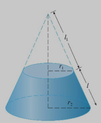
We can revolve a curve C around an axis to obtain a 3-dimensional shape C′. For our purposes, we will consider rotating C around the x-axis on the interval a≤x≤b for our derivation.
Just like in the 2-dimensional derivation for arc length, we will approximate C by partitioning it into n subintervals of equal length. Then, by rotating the line segments formed by the subintervals, we obtain an approximation for C′.
Figure 1. A diagram illustrating the method of approximating the shape of revolution of a Cartesian curve.
We can calculate the surface area of this shape by computing the lateral surface area of a frustum. *Note that the lateral surface area denotes the surface area of the frustum that does not include the circular bases.
Frustum?
A frustum is created when a cross section parallel to the cone's base (circle) splits the cone into two shapes: a cone above and a frustum below.
The lateral surface area of a frustum is
A=2πrl
Where r=21(r1+r2). *The proof of this will be left out for brevity. Search it up if you're interested!
Thus, we can approximate the surface area of the shape of revolution by summing the surface areas of the frustums. Note that the symbols used here are equivalent to the symbols used [[#Arc Length#Deriving for a Cartesian Curve|here]].
** Note that y is substituted for 2yi−1+yi for y because yi−1 and yi become infinitely close to each other as n tends to ∞. y can be substituted with F(x) when actually solving.
Surface Area of a Cartesian Curve
S=∫ab2πy1+(dxdy)2dx
Deriving for a Parametric Curve
The process here is identical to the parametric derivation for arc length.
You may not necessarily rotate a curve around the x-axis. Generally, you will be assigned to rotate around some line y=k (vertical) or x=h (horizontal). The formula is always similar, however. You simply replace y with a formula for the radius r.
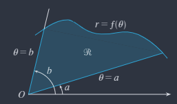
The polar coordinate system is an alternative to the Cartesian coordinate system, where a point P is represented by (r,θ). r is the length of the line segment between the poleO, which is typically the origin, and the point P. (We choose the variable r because it means radius). θ is the angle between the line segment and the polar axis. The polar axis is a ray that is typically equivalent to the positive x-axis.
Figure 2. A graph demonstrating polar coordinates. on the Cartesian plane.
Note that P(−r,θ)=P(r,θ+πn) for n∈Z and nodd. Also note that P(r,θ)=P(r,θ+2πn) for n∈Z.
Polar curves are essentially just a special form of parametric curves. Many of the same ideas/formulas for parametric curves will apply here too!
Cartesian to Polar
We can write a couple equations that represent the relationship between polar and Cartesian coordinates.
Based on the definitions of cosθ and sinθ, we can write
cosθ=rxsinθ=ry
It may help to refer to Figure 2 to see why these equations are true.
From this, it's easy to derive the following:
Polar → Cartesian Equations
x=rcosθy=rsinθ
Subsequently, we may derive the following:
Cartesian → Polar Equations
r2=x2+y2tanθ=xy
Finally, note that the equation of a polar curve is typically denoted as r=f(θ).
Symmetry
When sketching polar curves, recognizing symmetry can help significantly.
f(θ)=f(−θ)⟹
The curve is symmetric about the polar axis.
f(θ)=−f(θ)⟺f(θ)=f(θ+π)⟹
The curve is symmetric about the pole.
f(θ)=f(π−θ)⟹
The curve is symmetric about θ=2π (equivalent to y=x)
Derivatives
To derive polar curves, we essentially consider them as parametric. (Because, that basically is what they are!)
As a reminder,
x=rcosθy=rsinθ
Deriving,
dθdx=dθdrsinθ+rcosθdθdy=dθdrcosθ−rsinθ
Therefore,
dxdy=dθdxdθdy=dθdrcosθ−rsinθdθdrsinθ+rcosθ
Derivative for a Polar Curve
dxdy=dθdrcosθ−rsinθdθdrsinθ+rcosθ
For some θ=k:
dθdy=0∧dθdx=0⟹ Vertical Tangent.
dθdy=0∧dθdy=0⟹ Horizontal Tangent.
dθdy=dθdx=0⟹ Use L'Hôpital's Rule to calculate limθ→kdxdy.
Derivative at f(θ)=r=0
(Equivalent to a derivative at the pole)
dxdy=tanθ if dθdr=0
To find the 2nd derivative, we can follow the same steps as for a parametric curve. (Omitted for brevity).
10.4 Areas and Lengths in Polar Coordinates
Area
We define the area of a polar curve as the area swept out by the radius r=f(θ) between bounds a and b on θ. For instance,
We can approximate this area by summing several sectors of circles:
The area of a sector of a circle is
A=21r2θ
Therefore, we can approximate the area of the polar curve as
ΔAi=i=1∑n21[f(θi)]2Δθ
We take the limit as Δθ→∞⟹n→∞:
n→∞limi=1∑n21[f(θi)]2Δθ=∫ab21[f(θ)]2dθ
Therefore,
Area of a Polar Curve
A=∫ab21r2dθ
Arc Length
For the arc length of a polar curve, it suffices to repurpose the equation for the arc length of a parametric curve. Remember:
 We can approximate this area by summing several sectors of circles:
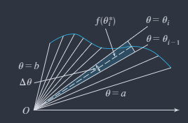 The area of a sector of a circle is