Chapter 3: Finite Markov Decision Processes

Markov decision processes (MDP) are the classical formalization of sequential decision making, where actions influence beyond just immediate state and reward.

3.1 The Agent-Environment Interface

In an MDP, the learner/decision-maker is called the agent, while what it interacts with is called the environment.

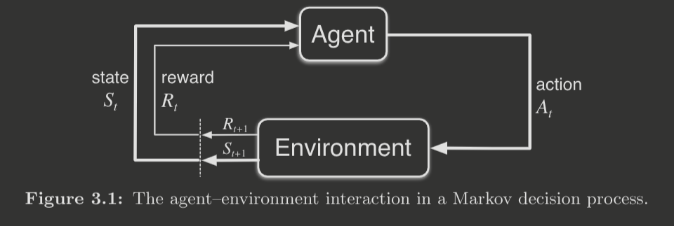
The iterative interactions between the agent and environment produce a trajectory

S_{0},A_{0},R_{1},S_{1},A_{1},R_{2},\dots

where the reward resulting from taking the action $A_{0}$ in state $S_{0}$ is $R_{1}$ , which is denoted as such because $R_{1}$ is really received at time step $t=1$ .

In a finite MDP, the number of possible states, actions, and rewards is finite, and all associated probability distributions are thus discrete. In particular, $S_{t},A_{t},R_{t}$ are all random variables described by discrete distributions.

The function

p(s',r \mid s,a)=\text{Pr}\{ S_{t}=s',R_{t}=r \mid S_{t-1}=s,A_{t-1}=a \}

fully describes the dynamics of the MDP. In other words, the probability of $S_{t},R_{t}$ depend solely on the preceding state and action, $S_{t-1}$ and $A_{t-1}$ . Critically, they do not depend on earlier states and actions. This quality of the MDP is known as the Markov property.

Using the four-argument dynamics function, one may calculate several other important expressions. For instance, the state transition probability function,

p(s'\mid s,a)=\sum_{r\in \mathcal{R}}p(s',r \mid s,a)

the expected reward function,

r(s,a)=\sum_{r\in \mathcal{R}}r\sum_{s'\in \mathcal{S}}p(s',r \mid s,a)

and the expected reward function for $(s,a,s')$ tuples,

r(s,a,s')=\sum_{r\in \mathcal{R}}r \frac{p(s',r \mid s,a)}{p(s'\mid s,a)}

As it turns out, this MDP framework is very flexible, and may be applied to many goal-directed learning problems!

3.2 Goals and Rewards

In RL, the goal of the agent is formalized/represented by a reward, a numerical signal that the agent will aim to maximize. This is known as the reward hypothesis: the goals are represented by the maximization of the expected value of the cumulative sum of a scalar signal (reward).

warning

The reward signal should not be used to express a prior describing how we think the agent should behave. It should only embody the problem goals.

3.3 Returns and Episodes

As aforementioned, the agent's goal is to maximize the cumulative sum of rewards. This is known as the return $G_{t}$ , defined as

G_{t}=R_{t+1}+R_{t+2}+\dots R_{T}

where $T$ is the final time step. Notably, $T$ is only finite when there is a sensible choice of a final time step, i.e. in which the agent-environment interaction process can naturally be broken into subsequences, or episodes. Typically, each episode will end when the agent reaches a terminal state. Note that the set of nonterminal states is denoted $\mathcal{S}$ and the set of all states (including terminal states) is denoted $\mathcal{S}^{+}$ . Moreover, $T$ is a random variable that varies between episodes. This problem setting is known as an episodic task.

Otherwise, when $T=\infty$ , i.e. there is no natural separation of the interaction process into episodes, this is known as a continuing task.

For continuing tasks, the above expression for the return is actually problematic! This is because the return can become infinite. Thus, a technique known as discounting is typically applied, with a discount rate $\gamma$ being included in the formula

G_{t}=R_{t+1}+\gamma R_{t+2}+\gamma^{2}R_{t+3}+\dots =\sum_{k=0}^{\infty} \gamma^{k}R_{t+k+1}

where $0\leq\gamma\leq1$ . If $\gamma<1$ , $G_{t}$ will be finite, provided the reward sequence $\{ R_{k} \}$ is bounded. If $\gamma=0$ , the agent is myopic in that it prioritizes only immediate rewards. Notably, with discounting, we may write a recursive formulation of the return.

G_{t}=R_{t+1}+\gamma G_{t+1}

3.4 Unified Notation for Episodic and Continuing Tasks

We note that the episodes in an episodic task are almost always identical, since they begin from the same starting state and the state transition probabilities are the same. Thus, rather than denoting the state at time $t$ for episode $i$ as $S_{t,i}$ , we assume henceforth we are just analyzing a single episode in isolation for an episodic task, and denote the state at time $t$ as just $S_{t}$ .

Additionally, we may frame an episodic task as a continuing task by creating an absorbing state that follows directly from a terminal state, and simply loops infinitely on itself with a reward of $0$ .

Thus, the combination of these two things allows the same exact notation for episodic and continuing tasks, and we may write

G_{t}=\sum_{k=0}^{\infty} \gamma^{k}R_{t+k+1}

for both types of tasks.

3.5 Policies and Value Functions

Practically all RL algorithms estimate value functions, functions that map a state or state-action pair to some estimate of its "value" (return). Value functions are defined with respect to a policy $\pi$ , which maps a state to a probability distribution over the action space, i.e. $\pi(a\mid s)$ .

Formally, the value function of a state $s$ under a policy $\pi$ , $v_{\pi}(s)$ , is the expected return of starting in $s$ and following $\pi$ thereafter.

v_{\pi}(s)=\mathbb{E}_{\pi}[G_{t}\mid S_{t}=s]=\mathbb{E}_{\pi}\left[ \sum_{k=0}^{\infty} \gamma^{k}R_{t+k+1}\mid S_{t}=s \right]

This is known as the state-value function for policy $\pi$ .

We may similarly define an action-value function for policy $\pi$ , $q_{\pi}(s,a)$ , which returns the expected return of starting in $s$ , taking action $a$ , and following $\pi$ thereafter.

q_{\pi}(s,a)=\mathbb{E}_{\pi}[G_{t}\mid S_{t}=s,A_{t}=a]=\mathbb{E}_{\pi}\left[ \sum_{k=0}^{\infty} \gamma^{k}R_{t+k+1}\mid S_{t}=s,A_{t}=a \right]

It's not possible to know the true value functions (at least, in most practical use cases), but they may be estimated based on the agent's interactions, by averaging the measured returns for each state/state-action pair. Such estimation methods are known as Monte Carlo methods because they average over many random data samples. We discuss such methods further in Chapter 5.

tip

It's usually not possible to keep averages for every single state when faced with extremely large state spaces. Instead, these functions are modeled using only much fewer parameters. (e.g. neural networks!)

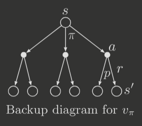
Notably, these value functions also satisfy recursive relationships.

\begin{align*} v_{\pi}(s)&=\mathbb{E}_{\pi}[G_{t}\mid S_{t}=s] \\ &= \mathbb{E}_{\pi}[R_{t+1}+\gamma G_{t+1}\mid S_{t}=s] \\ &= \sum_{a}\pi(a\mid s)\sum_{s'}\sum_{r}p(s',r \mid s,a)\Big[r+\gamma \mathbb{E}_{\pi}[G_{t+1}\mid S_{t+1}=s']\Big] \\ &= \sum_{a}\pi(a\mid s)\sum_{s',r}p(s',r \mid s,a)\Big[r+\gamma v_{\pi}(s')\Big] \end{align*}

this is known as the Bellman equation for the value function $v_{\pi}$ , and expresses the recursive relationship between the value of a state and the value of successive states. It may be visually displayed via a backup diagram, which diagrams the update or backup relationships for the value function.

Also, note the following relationship,

v_{\pi}(s)=\sum_{a}\pi(a\mid s)q_{\pi}(s,a)

which should hopefully be intuitive.

3.6 Optimal Policies and Optimal Value Functions

Solving an RL task, at its core, means finding an optimal policy. Notably, value functions define a partial ordering over policies, where a policy $\pi\geq \pi'$ if $v_{\pi}(s)\geq v_{\pi'}(s),\forall s \in \mathcal{S}$ . Consequently, there is always an optimal policy that is $\geq$ all other policies. We denote such a policy (though there may be multiple) as $\pi_{*}$ . Note that all optimal policies share the optimal state-value function, defined

v_{*}(s)=\underset{\pi}{\max}\ v_{\pi}(s),\ \forall s \in \mathcal{S}

Similarly, they share the optimal action-value function, defined

q_{*}(s,a)=\underset{\pi}{\max}\ q_{\pi}(s,a),\ \forall (s,a)\in \mathcal{S}\times \mathcal{A}(s)

Note that we may relate the two, i.e.

q_{*}(s,a)=\mathbb{E}[R_{t+1}+\gamma v_{*}(S_{t+1})\mid S_{t}=s,A_{t}=a]

We may also substitute the Bellman equation to derive the Bellman optimality equations, which is really just a mathematical formulation of the idea that "the value of a state under an optimal policy is equivalent to the expected return for the best action from that state."

\begin{align*} v_{*}(s) &= \underset{a\in \mathcal{A}(s)}{\max}\ q_{\pi}(s,a) \\ &= \underset{a}{\max}\ \sum_{s',r}p(s',r \mid s,a)[r+\gamma v_{*}(s')] \end{align*}

and

\begin{align*} q_{*}(s,a) \sum_{s',r}p(s',r \mid s,a)[r+\gamma \underset{a'}{\max}\ q_{*}(s',a')] \end{align*}

info

For finite MDPs, the Bellman optimality equations actually have unique solutions, and may be obtained by solving a system of nonlinear equations.

3.7 Optimality and Approximation

In practice, optimality is an ideal that agents can only approximate, not only because we usually have an imperfect model of the environment but also because the Bellman optimality equation is not easily solvable due to the massive state and action spaces.