7. Linear Programming and Reductions

7.1 Introduction

For a linear programming problem, we are provided a set of $n$ variables, to which we must assign real values such that they

1. Satisfy a provided set of linear equations/inequalities
2. Maximize/minimize a given linear objective function

We can draw the linear constraints on an $n$-dimensional hyperplane. The optimum solution, if it exists, will be located at a vertex of the $n$-dimensional polygon. This should naturally make sense; the optimum should make at least one of the inequalities reach its extremity.

Occasionally, the linear program can have no optimum, though. This occurs when the linear program is infeasible, i.e. the constraints are unsatisfiable, or unbounded, when it is possible to achieve arbitrarily small/large objective values.

Solving Linear Programs

All linear programs can be solved by the simplex method. Essentially, this algorithm starts at an arbitrary vertex, and greedily traverses to an adjacent vertex with a better objective value, until it reaches a vertex whose direct neighbors all have worse or equal objective value. Essentially, it hill-climbs up to the optimal vertex.

Why does local optimality imply global optimality? That is, why is the greedy algorithm correct? Consider the profit line passing through the vertex. Since all the vertex's neighbors lie below this line, the rest of the feasible polygon must also lie below this line because the polygon is convex. Simply consider the intersection of two inequalities in a 2D plane. The result must be a convex vertex.

Convexity
The notion of a "convex" polygon in terms of its angles does not extend well to higher dimensions. However, the formal definition of convexity extends to higher dimensions: a convex region is a set of points $S$ such that $\forall x,y\in S$, the line segment $x-y$ is entirely contained within the region.

Notably, all linear programs (LPs) can be reduced to one another via simple transformations. This is intuitively evidenced by how all LPs can be solved by the simplex algorithm.

Variants of LP

A general linear program has several degrees of freedom

1. It can be either a maximization or minimization problem
2. Its constraints can be equations and/or inequalities
3. The variables are often restricted to be nonnegative, but they can also be unrestricted in sign

Additionally, we discuss the simple transformations that can reduce all LP options to one another.

1. To transform a maximization problem to a minimization problem, or vice versa, negate all coefficients of the objective function.
2. 1. To turn an inequality constraint $\sum_{i=1}^{n}a_{i}x_{i}\leq b$ into an equation, we introduce a new variable $s$ and replace the inequality with the equation and inequality pair $\sum_{i=1}^{n}a_{i}x_{i}+s=b$ and $s\geq0$. This is called the slack variable for the inequality.
   2. To change an equality into an inequality, simple rewrite $ax=b$ into the pair of inequalities $ax\geq b$ and $ax\leq b$.
3. To transform a variable $x$ unrestricted in sign, we introduce two nonnegative variables $x^{+},x^{-}\geq0$ and replace $x$ with $x^{+}-x^{-}$. Thus, $x$ can take on any real value by adjusting these variables.

Applying these transformations enables us to reduce any LP to the standard form, which are described by the following constraints.

1. All variables are nonnegative
2. All constraints are equations
3. The objective function should be minimized

7.2 Flows in Networks

Maximum Flow

In this problem, we are provided a directed/undirected graph $G$ in which each edge has a capacity $c_{e}$. The goal is to find the maximum flow that can be sent from a source node $s$ to sink node $t$ such that the capacities of each edge are not exceeded. More formally, we define a flow within a network to be a set of variables $f_{e}$ for each edge $e$ in the network, satisfying the following properties.

1. It doesn't violate edge capacities, i.e. $0\leq f_{e}\leq c_{e},\ \forall e\in E$.
2. For all nodes $u$ besides $s$ and $t$, the amount of flow entering $u$ equals the amount of flow exiting $u$. That is, flow is conserved.

Then, the size of a flow is the total quantity sent from $s$ to $t$, which, by the conservation principle, is the quantity of flow leaving $s$. The maximum possible size across all valid flows is the maximum flow.

Notice how these constraints are just a linear program with several equations and an objective function (amount of flow leaving $s$) to be maximized.

Simplex Solution

Since maximum flow is an LP, we can apply the simple simplex solution to this problem! Of course, at the moment, we really only have a geometric intuition regarding the notion of an optimal solution. We won't formalize the generalized simplex algorithm yet. But, it turns out the maximum flow problem has a fairly concise interpretation of the simplex algorithm.

1. Start with zero flow.
2. Repeatedly choose an appropriate path from $s$ to $t$, known as an augmenting path, and increase the flow along the edges of this path as much as possible.*

As you may notice, this algorithm seems remarkably like a greedy algorithm! This should make sense, intuitively. Recall that the simplex algorithm is really just a greedy hill-climbing algorithm in the geometric interpretation.

You might notice that * for the second step though. There's a slight complication with a method; this greedy design is actually not always optimal, and is not the simplex algorithm for maximum flow. Instead, the simplex algorithm introduces one detail that makes it optimal: it allows new paths to cancel existing flows.

Thus, the simplex algorithm, for each iteration, finds a path from $s\to t$ whose edges $(u,v)$ can be categorized as one of two types.

1. $(u,v)$ in the original network, and is not yet at full capacity. Then, this edge can handle up to $c_{uv}-f_{uv}$ additional units of flow.
2. The reverse edge $(v,u)$ is in the original network, and there is some flow along it. Then, this edge can handle up to $f_{vu}$ additional units of flow.

These opportunities to increase flow can be imagined as a slightly modified graph $G^{f}$, known as a residual network, which represent the remaining flow that can be added along an edge. Thus, simplex is really just choosing an $s\to t$ path in this residual network.

Note that this algorithm is actually known as the Ford-Fulkerson method.

Minimum Cut

Maximum flow is actually the dual of another graph problem, minimum cut. The minimum cut problem presents the same graph as a maximum flow problem, except the goal is not to maximize flow, but minimize the total capacity of all edges from $L$ to $R$, where $L,R$ are two disjoint groups of vertices such that $s \in L$ and $t\in R$. This is known as an $(s,t)$-cut; thus, the minimum cut problem seeks to minimize the "size" of the $(s,t)$-cut.

Dual?
For an LP problem, its dual is a problem with equivalent solution, but phrased as the reverse optimization for the objective function. For maximum flow, it seeks to find the maximum size of a flow from $s$ to $t$. For minimum cut, its dual, it seeks to find the minimum total capacity across an $(s,t)$-cut. It's that simple!

In fact, this gives rise to a theorem known as

Max-Flow Min-Cut Theorem
The size of the maximum flow in a network equals the capacity of the smallest $(s,t)$-cut.

Efficiency

Though we have outlined the simplex algorithm for maximum flow, we have yet to discuss exactly how efficient it is.

Certainly, we can run a DFS or BFS algorithm on the residual graph for each iteration to find a valid path. But, how many times will this repeat? If we suppose all edges in the original network have integer capacities $\leq C$, then we can prove via induction that each iteration will increase the flow by an integer amount ($\geq1$). This is actually known as the

Integral Flow Theorem
If every capacity in the network is an integer, then the size of the maximum flow is an integer, and there exists a maximum flow such that each individual edge flow is integral.

As a direct result of this theorem, we can show that the algorithm will take at most $C$ iterations, and with a runtime of $\lvert E \rvert$ from DFS/BFS, the total runtime is $O(C\lvert E \rvert)$. But, we can do better!

Indeed, if the flows are chosen poorly, the simplex algorithm can take $O(C\lvert E \rvert)$ steps. However, it turns out using BFS to choose the flow each iteration actually bounds the number of iterations by $O(\lvert V \rvert \lvert E \rvert)$. Thus, the total runtime is $O(\lvert V \rvert \lvert E \rvert ^{2})$.

Edmonds-Karp Algorithm

The Edmonds-Karp algorithm, as described in the previous section, is just the simplex algorithm with BFS applied to the residual graph each iteration to identify a new flow. The key idea of using BFS is that, every time an augmenting path is found, one of the edges will become saturated. This edge may be revisited in the future, but, since BFS will always find paths in increasing order of edges, the number of edges between $s$ and this edge will increase by at least one each time it is revisited in an augmenting path. An augmenting path must, before visiting this edge, traverse at least one vertex, $s$, and can traverse at most $\lvert V \rvert-1$ vertices (all vertices except $t$). Therefore, this edge will reappear in an augmenting path at most $O(\lvert V \rvert)$ times. Thus, considering all edges, the number of augmenting paths that will be found by this algorithm is bounded by $O(\lvert V \rvert \lvert E \rvert)$. Since BFS has a runtime of $O(\lvert E \rvert)$, the total runtime is $O(\lvert V \rvert \lvert E \rvert ^{2})$.

$\square$

As a bonus, the Edmond-Karp algorithm works for even graphs with irrational edge capacities.

7.3 Bipartite Matching

Consider a bipartite graph whose two sets are equally sized and denoted $A$ and $B$. The Bipartite Matching problem considers if it's possible to form a matching of pairs between nodes in $A$ and $B$ such that every pair of nodes has an edge between them. This is known as a perfect matching, in graph theoretic terminology.

This problem can actually be reduced to a maximum flow problem! Create a source node $s$ with outgoing edges to all nodes in $A$ and a new sink node $t$ with incoming edges from all nodes in $B$. Then, assign each edge a capacity of $1$. Then, there exists a perfect matching $\iff$ the network has a flow whose size equals the number of pairs (which is the same as $\lvert A \rvert$ or $\lvert B \rvert$). There is one nuance to this reduction, though; the Integral Flow Theorem guarantees that, if the network has a maximal flow satisfying the above condition, then there exists a valid perfect matching since each individual edge flow is integral.

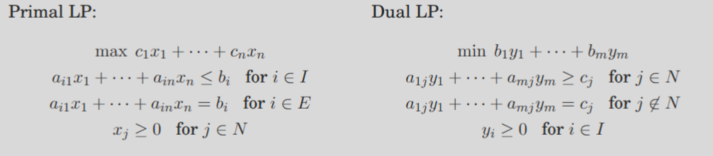
7.4 Duality

7.5 Zero-Sum Games

A zero-sum game is a game with one or more players in which the expected payout for each player is $0$. For instance, rock-paper-scissors (RPS) is a simple example of a zero-sum game.

For a zero-sum game, we can actually represent the situation with an LP. Consider two players $A$ and $B$ playing RPS. Each player gains $1$ point for a win, $-1$ for a loss, and $0$ for a draw. Both players, of course, seek to maximize their score. In particular, each player's goal also implies that they seek to minimize their opponent's score. WLOG, let us focus on $A$'s score. Then, $A$ will play to maximize $A$'s score, and $B$ will play to minimize $A$'s score.W

Well, if $A$ chooses to play completely randomly, then it turns out that $B$ can force an expected score of $0$ for $A$, no matter what $A$ does. Conversely, if $B$ chooses to play completely randomly, then it turns out that $A$ can force an expected score of $0$ for $B$. In other words, neither player can hope to increase/decrease the expected score of $A$ beyond $0$. Thus, the best each player can do is play randomly, with an expected score of $0$.

This remains the same even if one of $A$ or $B$ announces their strategy first! WLOG, let $A$ announce their strategy first. Intuitively, one would expect this to favor $B$, then. However, if both players play optimally (i.e. $A$ chooses the random strategy), $B$ cannot take advantage of this, and thus the expected score is still $0$. Remarkably, this is a consequence of linear programming duality, as you may have noticed from the maximization/minimization parallel. In essence, $A$, in their choice of strategy, is maximizing the minimum guaranteed expected average for themselves, while $B$ is minimizing the maximum guaranteed average of $A$'s score. In other words, $A$ is choosing the strategy such that it guarantees an expected score $\geq x$, where $x$ is maximal, regardless of $B$'s choice of strategy. $B$ is choosing a strategy such that it guarantees $A$'s expected score is $\leq y$, where $y$ is minimal, regardless of $A$'s choice of strategy.

Interestingly enough, in zero-sum games, $x=y$, i.e. there is a uniquely defined optimal strategy (across both players). This can be generalized to arbitrary games, and essentially illustrates the existence of mixed strategies that are optimal for both players and achieve the same value. This result is known as the minimax theorem, and is described by the equation

Note that when writing the LP for, WLOG, player $A$, one should seek to maximize some variable $a$ with constraints describing the idea that, no matter what strategy player $B$ picks, $A$'s expected score is $\geq a$. For instance, consider the zero-sum game described by the following matrix

Where the rows describe $A$'s choices and the columns describe $B$'s choices, and $M_{ij}$ describe the score $A$ receives if $A$ picks choice $i$ and $B$ picks choice $j$. Then, our LP has an objective function of $\mathrm{max}\ a$ and constraints of

Make sure this makes sense to you before moving on :)

7.6 The Simplex Algorithm

Finally, we describe the generalized simplex algorithm for solving LP problems. At a high level overview, the simplex algorithm receives an input of a set of linear inequalities, a set of variables in those inequalities, and a linear objective function, and finds the optimal feasible point using the follow strategy.

Let $v$ be any vertex of the feasible region. While there exists a neighbor $v'$ of $v$ with better objective value, $v\leftarrow v'$.

This is easy to visualize in 2D or 3D. But, what about in $n$ dimensions?

Notation

First, it's necessary to clarify some notations. Let $x_{i}\in \mathbb{R}$ represent the variables, where $1\leq i\leq n$. Any linear equation involving the $x_{i}$'s defines a hyperplane in the space $\mathbb{R}^{n}$. A linear inequality defines a half-space, all points that are either precisely on the hyperplane or lie on one side of it.

Meanwhile, a vertex is a unique point at which some subset of hyperplanes meet. This is always specified by at least $n$ inequalities. In particular, note that, with more than $n$ equations, we are guaranteed linear dependency; in other words, each vertex is actually specified by a set of precisely $n$ inequalities. By extension, we can note that two vertices are neighbors if they share $n-1$ defining inequalities.

*Notably, there can exist vertices that are generated by two different sets of inequalities. In particular, this occurs whenever some we have linear dependency for vertex. (which implies there are multiple sets of $n$ inequalities that can generate this vertex). These are degenerate vertices, and we will discuss how to handle them later. For now, assume all vertices are nondegenerate.

Algorithm

The algorithm, as previously described, consists of two simple steps.

1. Check the optimality of the current vertex, and halt if optimal.
2. Determine where to move next. Repeat.

Origin

Both steps are, in fact, easy if the vertex is at the origin. Consider a generic LP

Where $\mathbf{x}=[x_{1},\dots,x_{n}]^{T}$. Also, suppose the origin is within the feasible region. Then, it is certainly a vertex, as it is the unique point at which the $n$ inequalities $\{ x_{1}\geq0,\dots,x_{n}\geq0 \}$ reach their extremes, or are tight.

Task 1:
Claim: the origin is optimal $\iff$ $c_{i}\leq0,\forall i$.
Proof: If all $c_{i}\leq0$, then, considering that $\mathbf{x}\geq0$, it is impossible to increase the objective value, since each $x_{i}$ can only increase, and this will only result in $\mathbf{c}^{T}x$ decreasing.

$\square$

Task 2:
We can move to another constraint by increasing $x_{i}$ until another constraint is hit. In other words, we release the tight constraint of $x_{i}\geq 0$ (i.e., $x_{i}=0$ makes it tight), and thus allow increasing $x_{i}$ until some other inequality is now tight. This results in precisely $n$ tight inequalities (or more, but recall this can be reduced due to linear dependency).

Non-Origin

But what if we are at a non-origin vertex? Then, it suffices to transform the coordinate system such that this vertex is located at the origin.

Consider the $n$ tight inequalities that determine a non-origin vertex $\mathbf{v}$. Let the equation of one be denoted $\mathbf{a}_{i}\cdot \mathbf{x}\leq b_{i}$. Then, the distance from any point $\mathbf{x}$ to that hyperplane is $y_{i}=b_{i}-\mathbf{a}_{i}\cdot x$. These $n$ equations essentially define the distances $y_{i}$ as linear functions in $x_{i}$. The relationship can then be inverted to express the $x_{i}$'s as linear functions of the $y_{i}$'s, which consequently allows us to rewrite the entire LP in terms of the $y_{i}$'s (via substitution). If you consider the hyperplanes as the hyperaxes of the $n$-dimensional space, then $y_{i}$ are precisely the coordinates of any solution $\mathbf{x}$ in this new definition of the axes!

Notably, this LP with this new coordinate system has three properties:

1. It includes the inequalities $y\geq0$, which are just transformed versions of the inequalities defining $v$'s nonnegativity.
2. $v$ is the origin in $\mathbf{y}$-coordinate-space.
3. The cost function is now $\mathrm{max}\ c_{\mathbf{u}}+\tilde{\mathbf{c}}^{T}\mathbf{y}$, where $c_{\mathbf{u}}$ is the value of the objective function at $\mathbf{u}$ and $\tilde{\mathbf{c}}$ is the cost function transformed from in terms of $x_{i}$ to in terms of $y_i$.

Final Considerations

Starting Vertex

How do we find a starting vertex for the simplex algorithm? This is not entirely trivial because, in general, it's not necessarily true that the origin will be contained within the feasible region. (Otherwise, as previously stated, the origin is always a vertex).

Luckily, finding a starting vertex can itself be reduced to an LP. (And, fortunately, this LP has a known starting vertex).

Consider an LP in standard form, i.e.

First, make the RHS of the equations all nonnegative. IF $b_{i}<0$, just negate both sides of the $i$th equation. Then, create the following, separate LP:

• Add $m$ new variables $z_{1},\dots,z_{m} \geq 0$ such that $m$ is the number of equations.
• Add $z_{i}$ to the LHS of the $i$th equation in the original LP to produce $m$ equations for this LP.
• Let the objective to be minimized be $z_{1}+\dots+z_{m}$.

Note that, for this LP, the starting vertex $z_{i}=b_{i},\ \forall i$, and all other variables ($x_{1},\dots,x_{n}$) are set to $0$. Thus, we can subsequently just start the simplex algorithm.

The result is one of two possibilities. If $\mathrm{min}\ z_{1}+\dots+z_{n}=0$, then $z_{i}=0,\ \forall i$, and we get a starting feasible vertex of the original LP by just ignoring the $z_{i}$'s.

In contrast, if $\mathrm{min}\ z_{1}+\dots+z_{n}>0$, then the original LP is actually infeasible anyways! In other words, the original LP's equations required some nonzero $z_{i}$'s to be feasible, implying the original LP cannot be solved.

Degeneracy

As aforementioned, we previously assumed all vertices are nondegenerate. But, what if we do have degenerate vertices? Well, it could potentially result in vertices that seem like optimal solutions, since they are locally optimal, but are in fact suboptimal.

Naively, we can attempt to fix this by modifying simplex to detect degeneracy and continue moving to a different vertex despite lack of improvements in cost; however, this could result in an infinite loop. Instead, a smarter solution is to slightly perturb each $b_{i}$ to $b_{i}\pm\epsilon_{i}$, where $\epsilon_{i}$ is some tiny error value randomly chosen for each $i$. This ensures that there is no degeneracy in the entire system!

Unboundedness

What if an LP is unbounded in value? That is, the objective function can be made arbitrarily small/large when being minimized/maximized, respectively. In fact, simplex can be modified to detect this. When exploring the neighbors of a vertex, we can detect if removing a tight inequality and replacing it with another results in an undetermined system of equations with infinite solutions. In this case, simplex will simply halt.

Time Complexity

Let the LP have $n$ variables and $m$ inequality constraints. Consider an arbitrary vertex $\mathbf{u}$. By definition it is the unique point at which $n$ inequality constraints are tight. Each of its neighbors must share at least $n-1$ inequalities with it, and have $m$ degrees of freedom for the other inequality, so $\mathbf{u}$ has $O(mn)$ neighbors.

For each vertex $\mathbf{u}$, we must determine (1) if this vertex is more optimal and (2) if it is a true vertex. The first is simply a dot product. The second task is slow, however; it involves solving a system of $n$ equations in $n$ variables (i.e. satisfying the $n$ chosen inequalities as equations, to ensure they're tight) and checking the feasibility of the result. Applying Gaussian elimination to solve this has a runtime of $O(n^{3})$. This results in an overall runtime per iteration of $O(mn^{4})$. But, we can do better.

Recall the idea of moving $\mathbf{u}$ to the origin, providing a local view of the neighbors' optimality. It turns out that this transformation only has a runtime of $O((m+n)n)$; this is a result of exploiting the fact that the local view changes by just one defining inequality between iterations. Then, after transforming $\mathbf{u}$ to the origin, recall that the local view of the objective function is $\mathrm{max}\ c_{\mathbf{u}}+\mathbf{\tilde{c}}\cdot\mathbf{y}$. (Recall that $c_{\mathbf{u}}$ is the value of the objective function at $\mathbf{u}$, and can be calculated with just a dot product). Thus, it actually suffices to pick any $\tilde{c}_{i}>0$ (if there is none, the current vertex is optimal). And, since the LP has been rewritten in terms of $y_{i}$, it's much easier to determine how much $y_{i}$ can be increased before some inequality is violated. Thus, the total runtime for each iteration of simplex is just $O((m+n)n+mn)=O(mn)$. (Note that $m\geq n$, otherwise the LP is unbounded).

Then, how many iterations of simplex are there? There can't be more than $\binom{m+n}{n}$, since this is the maximum number of possible vertices. This is, in fact, exponential in $n$. And, in fact, it's not possible to produce a non-exponential upper bound; there do exist LPs in which simplex takes an exponential number of iterations! However, this does not typically occur in practice.