8. NP-Complete Problems
8.1 Search Problems
Throughout this book (a.k.a. throughout these notes), we have discussed efficient algorithms that frequently search for a desired solution in polynomial runtime among an exponential search space. However, not all such problems can be efficiently solved.
SAT
Consider the SAT or Satisfiability problem. We are provided a Boolean formula in conjunctive normal form (CNF), which is composed of the logical and (conjunction) of several clauses, each the logical or (disjunction) of several literals, where a literal is either a Boolean variable or the not of one. For instance, here's an example of a CNF formula.
The SAT problem asks us to find an assignment of the Boolean variables such that this statement is true or else report that none exists. This problem, in particular, does not have a solution. But, in general, it's difficult to efficiently find a solution: the search space is , where is the number of variables, and there is no known efficient algorithm for the general SAT problem.
Note, though, that the SAT problem is again a typical search problem. Provided an instance (CNF formula), we are asked to find a solution or report that none exists. In particular, a search problem must also have the property that 's validity as a solution for can be checked in polynomial runtime. Formally,
A search problem is specified by an algorithm that takes two inputs, an instance and a proposed solution , and runs in time polynomial in . We say is a solution to
There do, however, exist two notable variants of SAT that can be efficiently solved. If each clause contains at most one positive literal (i.e. is positive, is negative), then the Boolean formula is a Horn formula. We discussed an efficient greedy solution to this problem in Section 5.3. Meanwhile, if all clauses have at most two literals, then the problem is called a 2SAT problem, and it can be solved in linear time by identifying the SCCs of a graph constructed from the instance. (Recall the efficient algorithm we derived for this in Section 3.4).
Conversely, some problems that seem easier than the general SAT problem are still hard to solve! If all clauses have at most three literals, we have what is known as a 3SAT problem—and this problem is actually just as hard as the general SAT problem!
TSP
In the Traveling Salesman Problem, we are provided an instance with vertices , all pairwise distances between them, and a budget . The desired solution is a tour, a cycle that passes through each vertex precisely once, of total cost at most (or else report none).
Typically, TSP is actually discussed as an optimization problem, in which the shortest possible tour is desired. However, here we frame it as a search problem. Why? So that we can compare TSP with other search problems. Search problems are such a general description of problems that other types of problems can often be framed as search problems, like for TSP. More accurately, in this instance, the optimization version of TSP (which we will call Min-TSP henceforth) reduces to TSP. In essence, this means that solving Min-TSP is at least as hard as solving TSP. For TSP, this intuitively is because we can find a solution for Min-TSP by binary searching the budget for TSP. We formalize this notion later.
Also, interestingly enough, one might note that Min-TSP seems like a difficult analogue to the minimum spanning tree problem, which we have developed efficient greedy algorithms for in Section 5.1. In essence, Min-TSP just replaces the minimum spanning tree with a more difficult constraint—a tour. This simple change results in an exponentially harder problem (literally!).
Eulerian and Rudrata/Hamiltonian Paths
Now, we turn to another sibling pair of graph problems.
Several hundred years ago, Euler sought to solve a problem—given a graph , does there exist a path in the graph such that each edge in the graph is traversed exactly once? It turns out that this problem has an exceedingly elegant solution—there exists a Eulerian path all vertices, except for two (start, end), must have even degree.
As before, let's now define this problem as a search problem. The Eulerian path problem provides an instance with a graph , and the desired solution is a valid Eulerian path. We won't discuss the solution in detail—but, it follows from Euler's observation that the search problem can also be solved in polynomial time.
Before Euler solved his namesake graph problem, though, Rudrata sought to solve another, very similar problem. Given a graph , does there exist a path in the graph such that each vertex in the graph is traversed exactly once? Again, we frame this problem as a search problem, too. The Rudrata path (also known as Hamiltonian path) problem provides an instance with a graph , and the desired solution is a valid Rudrata path.
This seems very similar to Euler's problem! Despite this, there is no known efficient algorithm to solve the Rudrata path problem.
You may have heard the more familiar namesakes Eulerian cycle or Hamiltonian cycle, rather than the path variants described above. Well, as we will see later, these problems are effectively equivalent to their path variants!
Cuts and Bisections
Recall our minimum cut problem from Section 7.2. As aforementioned, a cut is a set of edges whose removal leaves a graph disconnected. We can generalize the minimum cut problem to a search problem: given an instance with a graph and budget , the desired solution is a cut with at most edges.
Of course, the minimum cut problem has a polynomial time algorithm. However, there exist other cut problems that, as far as we know, cannot be efficiently solved! In particular, the Balanced Cut problem is a variant of the general cut search problem: given an instance with a graph and budget , the desired solution is a partition of vertices into sets such that and there are at most edges between and .
Balanced cuts actually have many important applications, such as clustering! However, its intractability forces such applications to use efficient approximations of solutions.
Integer LP
We discussed linear programming extensively in Section 7, and noted that, though the simplex algorithm does not always run in polynomial time, there does exist a polynomial algorithm for linear programming—at least, when the solutions are allowed to be anything in . When we constrain solutions to be in , i.e. Integer Linear Programming (ILP), the problem becomes intractable!
More formally, let us frame ILP as the following search problem: given an instance of an matrix and an -vector , the desired solution is a nonnegative integer vector satisfying .
There is additionally a special case of ILP that is just as hard, known as Zero-One Equations (ZOE). In particular, we constrain to have entries of only either or , to be a vector of only 's and 's, and (the -vector of all 's).
Three-Dimensional Matching
Recall the bipartite matching problem we discussed in Section 7.3, which can be efficiently solved with the Edmonds-Karp algorithm. There exists an intractable generalization of this known as 3D Matching: given an instance with boys, girls, and pets, and compatibilities among them described by a set of triples of the form (,,), the desired solution is a set of disjoint triples that is a subset of the set of compatible triples.
Independent Set, Vertex Cover, Clique
The Independent Set problem: given an instance with a graph and an integer , the desired solution is a set of independent vertices, i.e. no pair of vertices have an edge between them. Recall from Section 6.7 that, via dynamic programming, we could efficiently solve this problem on a tree. However, for general graphs, there exists no known polynomial-time algorithm!
The Vertex Cover problem: given an instance with a graph and budget , the desired solution is a set of vertices such that each edge in the graph is adjacent to at least one vertex in this set. This is actually a special case of the Set Cover problem: given an instance with a set , , and a budget , the desired solution is a set of subsets such that their union is . Note that we briefly discussed a greedy approximation of a solution to the minimum size Set Cover problem in Section 5.4. Regardless, these problems are both intractable.
We'll discuss why this is the case soon... sorry for the suspense :P
is all boys, girls, and pets, the subsets are precisely the triples of , and the budget is .
Finally, the Clique problem: given an instance with a graph and goal , the desired solution is a set of vertices such that all possible edges between them are present (i.e. these vertices form a fully connected subgraph in ).
Longest Path
Recall from Section 4 that the shortest path problem can be solved efficiently using Dijkstra's Algorithm or Bellman-Ford's Algorithm. What about the analogue, longest path? Formally, given an instance with a graph whose edges are assigned nonnegative edge weights, two vertices , and a goal , the desired solution is a simple path from with total weight at least .
It might seem that simply negating all the edge weights, and running a shortest path algorithm that can deal with negative weights on this graph would efficiently solve this problem. However, the issue with this is that these algorithms do not actually find the shortest simple path on a graph with a negative cycle! And, a negative cycle can certainly be created since all edges in the longest path problem are nonnegative (so negating them will make them all nonpositive). And, in fact, there is no known polynomial time algorithm to solve the longest path problem.
Knapsack and Subset Sum
We now frame knapsack as a search problem: given an instance with a weight capacity , a goal , and a set of items with weights and vales , the desired solution is a set of items whose total weight is at most and whose total value is at least .
In Section 6.4, we discussed algorithms for solving the knapsack problem that run in time. Is this polynomial time, though? Well, not in , since can be arbitrarily large. If we try and remove from the time complexity, then it turns out that the best we can do is , checking all possible subsets of items. So, there isn't actually a polynomial time algorithm for knapsack!
Actually, we can derive a polynomial time for a somewhat contrived variant: Unary Knapsack, in which we represent, e.g., as . This isn't too useful, but, yes, this does have a polynomial time algorithm, due to the limitation this places on .
Meanwhile, an equally hard special case of knapsack is also of particular interest. The Subset Sum problem: given an instance with integers and a capacity , the desired solution is a subset of the provided integers that add up to precisely . Note that this is a special case of knapsack where for each item and , and that the constraints and in knapsack is equivalent to here.
Why is this special case of knapsack interesting, if it's equally as hard as knapsack? The point is simplicity; as we'll soon see, exploring reductions between problems is much easier with simpler problems like Subset Sum.
8.2 NP-Complete Problems
Tractability
Consider the following table of sibling hard vs. easy search problems (we'll discuss what NP-Complete and P are soon).
| Hard (NP-Complete) | Easy (P) |
|---|---|
| 3SAT | 2SAT, Horn SAT |
| TSP | MST |
| Longest Path | Shortest Path |
| 3D Matching | Bipartite Matching |
| Knapsack | Unary Knapsack |
| Independent Set | Independent Set (Trees) |
| ILP | LP |
| Rudrata Path | Eulerian Path |
| Balanced Cut | Minimum Cut |
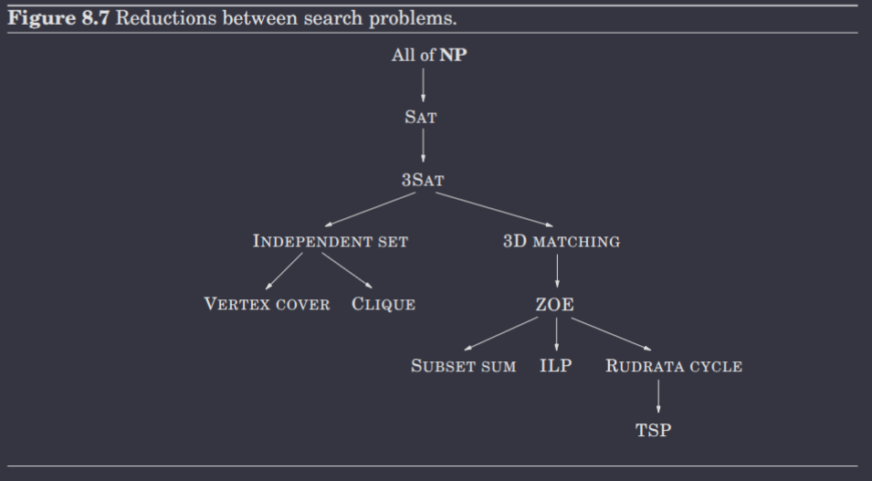
On the right are easy problems, which are all easy for a variety of different reasons/algorithms (DP, greedy, etc.). On the left, though, are all hard problems, which researchers have been unable to efficiently solve over many, many years. The fascinating thing about these hard problems is that they are all difficult for the same reason! This may seem incredibly counterintuitive—they're all different problems, and vary widely. How could they possibly all be the same difficulty?! Well, as we'll soon discuss, these are actually all the same problem! That is, these problems are all equivalent; as we'll soon discuss, these problems can all be reduced to each other.
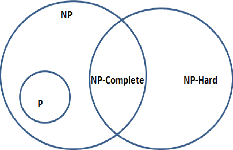
P, NP
No, P/NP does not mean Pass/No Pass here. and are what's known as complexity classes. You've probably heard of these before too; perhaps in the context of the Millennium Problems—each problem within this set of problems has a $1 million bounty, and one such problem is proving (or disproving!) that . But what do these actually mean?
Formally, denotes the class of all search problems. We formally defined these [[#8.1 Search Problems|above]], but, in short, a search problem must possess an efficient algorithm to check if a solution is valid for a given instance . Efficient, here, means polynomial in . Note that this includes both intractable (e.g. 3SAT) and tractable (e.g. 2SAT) problems.
, meanwhile, denotes the class of all search problems that can be solved in polynomial time. Importantly, . (And thus, the Millennium problem essentially seeks to prove the conjecture ; generally speaking, we assume is true. Proving the contrary would mean that all these "hard" problems are solvable in polynomial time!).
Reductions
Well, now that we've defined our complexity classes, and now that we've clarified our assumption that , how do we prove that these hard problems have no efficient algorithm? This is done via reductions, transformations that show one problem is at least as hard as another. Researchers have leveraged reductions to show that all the problems on the left side of the above table are essentially the exact same problem, as aforementioned. What's more, they have shown that these problems are in fact the hardest search problems in . If any of these problems has a polynomial time algorithm, then every problem in would have a polynomial time algorithm.
Let's first formalize the notion of a reduction. A reduction from search problem to search problem is a pair of polynomial time algorithms such that
- transforms any instance of into an instance of
- transforms any solution of for into a solution of for . Or, if has no solution for , then it can be concluded that has no solution for .
Note how this reduction from effectively shows that is at least as hard as , since, if there exists a polynomial time algorithm for , there naturally exists a polynomial time algorithm for derived from 's via the reduction.
Now, we can formally define the class of the hardest search problems, too (the left side of the above table). A search problem is -Complete if all other search problems reduce to it.
Composition of Reductions
One final note about reductions is that they compose, i.e. and implies . This should hopefully make sense intuitively.
NP-Hard?
You might have heard of the term -Hard to refer to the hardest problems in computer science. So what's this -Complete term then?
Well, -Hard is actually yet another complexity class. -Hard denotes the class of all problems at least as hard as -Complete problems.
Not quite. -Complete denotes the class of the hardest search problems. There exist non-search problems at least as hard as those in -Complete—those are the ones in -Hard.
Note that, similar to how , -Complete -Hard. Also, -Hard is not a subset of ! Remember that denotes the class of all search problems. Thus, -Complete denotes the intersection of -Hard and .
Finally, you should hopefully be able to understand the following diagram!
Factoring
Factoring is a famously difficult search problem: given an integer , the desired solution is the prime factorization of . So, does Shor's Algorithm, i.e. a polynomial time quantum algorithm to prime factorize a number, solve all of ?
Not quite. In fact, factoring isn't one of the hardest problems in , i.e. it isn't an -Complete problem! One critical difference between factoring and the -Complete problems is that, for factoring, there is no "or else" clause—there is always a prime factorization for . In any case, factoring is within , but not -Complete. So, while quantum computers are able to efficiently solve factoring, it still remains to be seen whether or not all of can be solved efficiently by quantum computers! (Though, current research seems to indicate that it is very likely that this is not the case).
8.3 Reductions, Reductions, Reductions
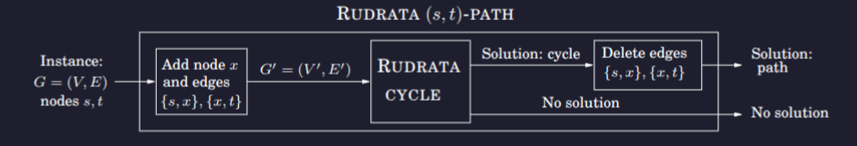
Rudrata -Path Rudrata Cycle
Consider adding an additional vertex and two new edges and to the graph to produce . Then, any Rudrata cycle of the graph must contain the edges and . Proving this reduction's validity requires showing that it works for when the Rudrata Cycle problem has a solution and when it does not. Moreover, it must be shown that the preprocessing and postprocessing functions take polynomial time.
1. Existing Solution
Then, the Rudrata -Path problem must also have a solution. Consider that removing the added edges from the Rudrata cycle of produces the Rudrata path from in , as desired, since the other half of the cycle, , must traverse through (otherwise would not be visited by the cycle, and thus it would not be a valid Rudrata cycle for ).
2. No Solution
It's typically easier to show the contrapositive, for this case. For this instance, it requires proving that, if there exists a Rudrata -path in , then there also exists a Rudrata cycle in . This is trivially true; just add the edges to the Rudrata path to close the cycle.
3. Preprocessing & postprocessing
The preprocessing step just requires adding one node and two edges. The postprocessing step just requires removing two edges. Thus, these steps are clearly polynomial time.
Thus, solving the Rudrata Cycle problem is at least as hard as the Rudrata -Path problem. In other words, the Rudrata -Path problem reduces to the Rudrata Cycle. Below is a diagram that illustrates the reduction visually.
It's also possible to reduce in the other way, i.e. Rudrata Cycle Rudrata -Path. In other words, this pair of reductions show that these two problems are essentially the same problem.
3SAT Independent Set
This reduction is most succinctly described by the following diagram.
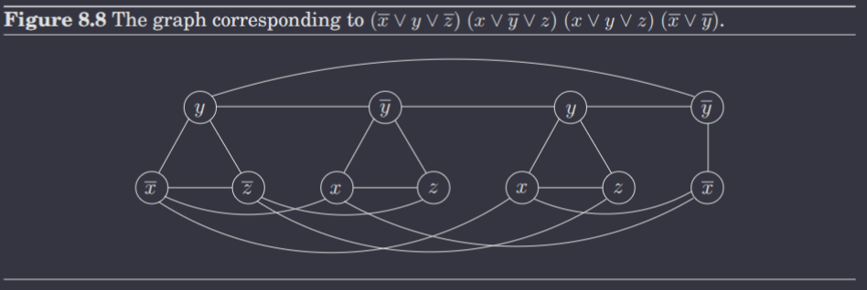
In essence, the idea is that precisely one literal is chosen to be true in every clause, in order to make that clause true. Moreover, each node, WLOG , is connected directly to all of its negations, i.e. all nodes . This ensures that, if is chosen in a clause, is never chosen in any other clause, since this would violate the property of an independent set. Note that multiple literals in a clause can actually be true, despite the graph ensuring only one is chosen for the independent set! This is okay, since we don't need to represent all literals that are true within a clause; only one needs to be true (in the independent set) to make that clause true. (Note that including one node in the independent set, i.e. marking it as true, will not immediately add all other nodes to the independent set; rather, it will simply preclude all nodes from being part of the independent set).
SAT 3SAT
This is an example of an interesting yet common reduction: reducing a problem to a special case of itself. In essence, this shows that the hardness of the problem is equivalent to the hardness of a special case.
The entire reduction relies on a single trick. Consider any clause in the SAT problem with more than three literals, i.e.
where . Then, we can rewrite this as a set of 3SAT clauses
The conversion is clearly polynomial in (and thus polynomial in the SAT instance 's size, ), and the conversion from 3SAT back to SAT is clearly (since all variables were already solved for in 3SAT).
We can go even further than this, though. We can additionally reduce the 3SAT problem to a variant such that no variable appears in more than three clauses. Consider any variable that appears in clauses. Then, replace its th appearance with , and add the clause
Note how appears thrice, twice in the above expression and once in its original clause.
Independent Set Vertex Cover
We alluded to this reduction earlier in [[#8.1 Search Problems#Independent Set, Vertex Cover, Clique|Section 8.1]]. Consider that a set of nodes is a vertex cover of graph is an independent set of .
Forward Direction:
We proceed via proof by contraposition. Let not be an independent set of . Then, such that the edge . Then, , and thus the edge is not covered by . Therefore, is not a valid vertex cover.
Backward Direction:
Again, we can prove this by contraposition. The details are left as a (hopefully easy) exercise to the reader! >:)
Independent Set Clique
Define the complement of a graph to be , where consists of all edges not in . Then a set of nodes is an independent set of is a clique of . That is, the nodes in have no edges between them in all possible edges exist between them in . This should hopefully make sense intuitively.
3SAT 3D Matching
This is a very unintuitive reduction. But, I'll do my best to explain the transformation.
Consider the following 3D Matching diagram, where each triangle node represents a triple.
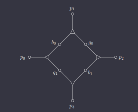
Suppose and are not involved in any other triples. Some of the pets must belong to other triples, of course, since at most two triples can be chosen here (and thus at most two pets can be "used up" here). In fact, precisely two pets must be "used up" here, since, in order for a perfect matching, must all be "used up" in this diagram, since they are not involved with any other triples.
Consider choosing the triple . Then, this forces the other triple in this diagram to be . Similarly, choosing the triple forces the other triple to be . Therefore, any matching involving this gadget must include either both and or both and . In other words, this gadget behaves like a Boolean variable!
So, to transform an instance of 3SAT into an instance of 3D Matching, we first create a gadget for each variable. Let the nodes for a variable be denoted . We will let be denoted by the case where is matched with girl , and be denoted by the case where is matched with .
Now, consider a clause, e.g. . For each clause, we introduce a new boy and new girl . We will associate each with three triples, one for each literal in the clause. In essence, we want this boy and girl pair to be matched with a single pet in one of the literals' gadgets, such that this match implies that this literal was chosen to be true.
For this clause, we can have . For , we form the triple . This is because, if is chosen to be true, then would be taken in the gadget. Then, the triple can be included in the 3D Matching, effectively marking that makes clause true. In contrast, if is chosen to be false, then would be taken in the gadget is not used to make the clause true. We extend this to the other two literals, i.e. has the triple and has the triple .
Additionally, we have to ensure that, for every occurrence of a literal in clause , there is a different pet to match with and . For instance, if a literal is used in 5 different clauses, we won't have enough pets to match with for each clause ! However, recall that we actually showed a reduction from 3SAT to a special case in which each literal appears in at most two clauses. Therefore, if we first reduce 3SAT to a special case, we can ensure each literal appears at most twice, in which case we actually do have enough pets—if a variable , we have two pets and that can each be matched in clauses, and if , we have and .
I was confused about this too. Actually, the earlier reduction showed that each variable appeared in at most three clauses. Notably, though, in the expression derived to ensure , each variable was used once as and once as . Meanwhile, the original clause contains one of or . Therefore, each literal, i.e. and are the literals, appears at most twice. Confusing, I know; I wish the book explained this.
We're almost done now. The last thing we need to ensure is that no pet is left unmatched. For instance, consider a variable that is used only in one clause—it'll be left with an unmatched pet, which isn't allowed in 3D Matching! More precisely, with variables and clauses in 3D SAT, precisely pets will be left unmatched. Thus, it suffices to simply add boy-girl couples that can match with every pet, and have them take up the remaining pets!
Each variable's gadget will have two pets that are not matched within the gadget itself. Each clause will take precisely one pet. Thus, pets left unmatched. Note that always since each variable will appear at most thrice, and there are at least two literals in every clause.
3D Matching ZOE
For each triple, create a variable , where means the triple was chosen. Our vector . Then, for each boy/girl/pet, let the triples containing it are . Then, we can set a constraint
since each boy/girl/pet can be included in at most one triple. Then, the rest is just solving the corresponding ZOE problem,
where each column of corresponds to a triple, and each row corresponds to a boy/girl/pet.
ZOE Subset Sum
This is a reduction between two special cases of ILP, and is literally just based on the fact that vectors can essentially act as binary representations of a number!
For instance, consider the ZOE problem with matrix
Think of the columns as binary; then, effectively,
. Then,
reduces to the subset sum problem where we are searching for a subset of that sums to .
Well, not quite. There's still one more consideration—carries from addition can result in a valid solution for Subset Sum but an invalid solution for ZOE. To fix this, we can slightly modify the transformation: instead of thinking of the column vectors as integers in base , we consider them as integers in base . Therefore, this ensures that carries never occur, and thus a solution to Subset Sum is always a solution to ZOE.
ZOE ILP
As aforementioned, ZOE is a special case of ILP. Then, this effectively means that ZOE reduces to ILP, since being able to solve ILP in polynomial time trivially equates to being able to solve ZOE in polynomial time, since there isn't even a transformation required.
ZOE Rudrata Cycle
This transformation is complex and fairly long, so I will attempt to explain it concisely as best as I can.
First, we will try to reduce ZOE to a generalization of Rudrata Cycle: Rudrata Cycle with Paired Edges, and then we will reduce this generalization to Rudrata Cycle. (Recall that this is valid since reductions are transitive).
ZOE Rudrata Cycle with Paired Edges
In Rudrata Cycle with Paired Edges, a graph and a set comprise the provided instance. The desired solution is a cycle that visits all vertices once and for every pair of edges , traverses precisely one of the two.
Now, consider the structure of a ZOE problem. We have variables that can either be or , and equations , where . For variable , we create a component consisting of two nodes and two edges and between these two nodes, where the Rudrata cycle traversing corresponds to , and it traversing corresponds to . For equation , we create a component consisting of two nodes and edges , where e.g. the Rudrata cycle traversing corresponds to the variable in equation . Then, we compose these components as shown in the diagram below.
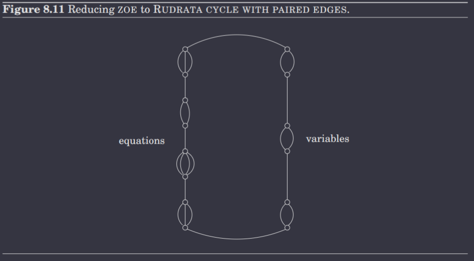
Then, for every equation, for every variable appearing in it, we add to the pair where corresponds to the edge representing in the equation and corresponds to the edge represent . This ensures that if , it's never used as the value in any equation. Therefore, ZOE reduces to the Rudrata Cycle with Paired Edges problem.
Rudrata Cycle with Paired Edges Rudrata Cycle
This transformation can be summed up in a single diagram.
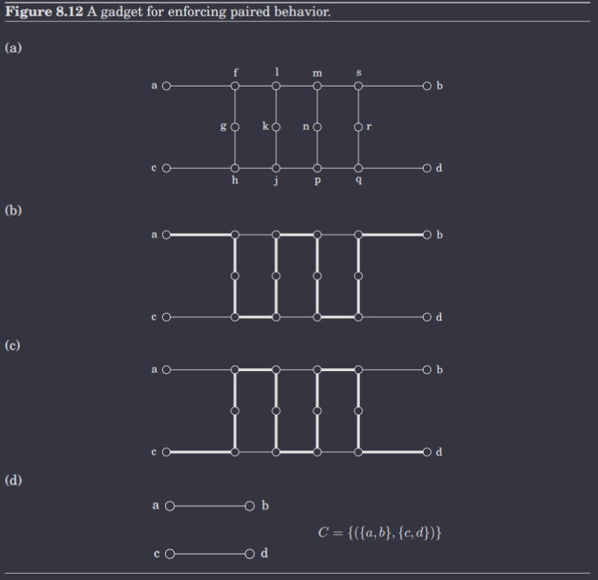
In essence, by replacing every pair of edges with this gadget, we ensure that only one of is traversed. Thus, the Rudrata Cycle with Paired Edges problem reduces to the Rudrata Cycle problem, and by the transitivity of reductions, ZOE reduces to the Rudrata Cycle Problem.
Then we can simply concatenate all of its gadgets together. Make sure you see why this works!
Rudrata Cycle TSP
Given a graph , construct a TSP where the set of cities is precisely the same as , the distance between cities and is if and otherwise is , for some . The budget is .
If has a Rudrata cycle, then the same cycle is also a tour within the budget of the TSP instance, clearly. Conversely, if has no Rudrata cycle, then there is no solution, as the cheapest possible TSP tour has a cost (since it traverses at least one edge that doesn't exist in , and thus has length ).
Varying can lead to two interesting results. If , then this TSP instance actually satisfies the triangle inequality, which produces a special case of TSP that, as we will discuss in Section 9, can be efficiently approximated.
Conversely, if is sufficiently large, then it has the property that it either has a solution of cost or has a solution of cost . Critically, there are solutions with cost such that . This is known as the gap property, and implies that unless , there exists no efficient approximation algorithm.
Any Problem in SAT
ts too hard... TL;DR is Any Problem in Circuit SAT SAT.
Summary
Now, you should hopefully understand the tree of reductions shown in the below diagram :)
Aside: Unsolvable Problems
For all -Complete problems, there at least exists some algorithm to solve each, even if intractably so. For such problems, there is no existing algorithm at all! One such problem is the arithmetical version of SAT, where the provided instance is a polynomial equation in many variables and the desired solution is a satisfying assignment of the variables. Another very famous unsolvable problem is the halting problem.