Lecture 10: Advanced Policy Gradients: Part 2

Mathematical Shortcuts So Far

When rewriting the importance sampling policy gradient formula with causality, we $(1)$ removed the $B$ term, i.e.

Which corresponds to essentially using the advantage with respect to the policy $\pi_{\theta}$, $\hat{A}^{\pi_{\theta}}$, instead of the advantage with respect to the policy we're improving, $\hat{A}^{\pi_{\theta'}}$. That is, leaving in the $B$ term uses importance sampling to correct the advantage according to the importance sampling ratio between the two distributions; removing it means using the advantage without adjusting for the difference in distribution.

We also replaced term $A$ with a state-action marginal, which is equivalent under expectation,

and $(2)$ ignored the mismatch between the state distributions of the two policies.

In short, there are two shortcuts:

1. Incorrect advantage
2. Incorrect state distribution

Policy Iteration $\to$ Policy Gradient (Incorrect Advantage)

Policy gradient, notably, may be viewed as policy iteration.

1. Estimate $\hat{A}^{\pi}(\mathbf{s}_{t},\mathbf{a}_{t})$ for current policy $\pi$.
2. Use $\hat{A}^{\pi}$ to produce an improve policy $\pi'$.

We can formalize this by using an alternate objective

where we define

we will attempt to prove this claim of equality.

Proof.

Reasoning for each step:

1. Substitution of given expression.
2. The initial state distribution is the same for any policy.
3. Equivalent expression.
4. Equivalent expression (flips sign of second term, exploits $\infty$).
5. Definition of $J(\theta')$.
6. Combining expectations ($\tau$ sampled from same distribution).
7. Definition of advantage function $A^{\pi_{\theta}}$.

So what does this really mean in the context of policy iteration? With the objective $J(\theta')-J(\theta)$, we are maximizing the expectation of our returns under policy $\pi_{\theta'}$, formulated via the estimated advantage, according to the advantage function of $\pi_{\theta}$, of the discounted trajectories sampled from $\pi_{\theta'}$.

Now, we note the following expansion.

where the inner expectation of sampling actions was changed to sample from the $\pi_{\theta'}$ distribution to the $\pi_{\theta}$ distribution, with the added correction of the importance sampling factor $\frac{\pi_{\theta'}(\mathbf{a}_{t},\mathbf{s}_{t})}{\pi_{\theta}(\mathbf{a}_{t},\mathbf{s}_{t})}$. Thus, we've proved that using the advantage function of $\theta$, not $\theta'$, is okay! (The optimization of $J(\theta')-J(\theta)$ is the same as the optimization of $J(\theta')$ by itself since $J(\theta)$ is a constant as the old policy's parameters $\theta$ are a constant).

Incorrect State Distribution

We'd like for

because we'd like to sample from our $\theta$ distribution, and not have to generate new samples from our $\theta'$ distribution. We will denote the RHS as $\bar{A}(\theta')$, and we will note that equality is generally not true unless $p_{\theta}=p_{\theta'}$; hence we want to show when exactly we may allow this approximation.

Claim: $p_{\theta}(\mathbf{s}_{t})\approx p_{\theta'}(\mathbf{s}_{t})$ when $\pi_{\theta}\approx \pi_{\theta'}$, for some notion of "closeness" or $\approx$.

Naturally, such a claim seems obvious. We will proceed to formalize this notion, though

Proof.
Case 1: $\pi_{\theta}$ is deterministic.
Let $\mathbf{a}_{t}=\pi_{\theta}(\mathbf{s}_{t})$. Let $\pi_{\theta'}\approx \pi_{\theta}$ if $\pi_{\theta'}(\mathbf{a}_{t}\neq \pi_{\theta}(\mathbf{s}_{t})\mid \mathbf{s}_{t})\leq\epsilon$ for some small $\epsilon$. Actually, we can apply techniques from Lecture 2 to this proof; in particular, the proof about distributional shift for behavioral cloning. In fact, the rest of the proof is precisely identical! This allows us to conclude that $D_{\text{TV}}(p_{\theta'},p_{\theta})=\frac{1}{2}\sum_{\mathbf{s}_{t}}\lvert p_{\theta'}(\mathbf{s}_{t})-p_{\theta}(\mathbf{s}_{t}) \rvert\leq\epsilon t$.

This isn't quite a great bound yet, though, because the total variation divergence between the two distributions is linear in the horizon length.

Case 2: $\pi_{\theta}$ is an arbitrary distribution (may be stochastic).
This is the more general case. Let $\pi_{\theta'}\approx \pi_{\theta}$ if $D_{\text{TV}}(\pi_{\theta'}(\mathbf{a}_{t}\mid \mathbf{s}_{t}),\pi_{\theta}(\mathbf{a}_{t}\mid \mathbf{s}_{t}))\leq\epsilon$. We first consider a useful lemma:

If $D_{\text{TV}}(p_{X}(x),p_{Y}(x))\leq\epsilon$, there exists $p(x,y)$ such that $p(x)=p_{X}(x)$, $p(y)=p_{Y}(y)$, and $p(x=y)=1-\epsilon$.

In other words, $p_{X}(x)$ "agrees" with $p_{Y}(y)$ with probability $1-\epsilon$. In the context of our proof, $\pi_{\theta'}(\mathbf{a}_{t}\mid \mathbf{s}_{t})$ takes a different action than $\pi_{\theta}(\mathbf{a}_{t}\mid \mathbf{s}_{t})$ with probability at most $\epsilon$. (In practice, we enforce this constraint).

This lemma actually allows us to do the exact same thing as before, i.e. show that $D_{\text{TV}}(p_{\theta'},p_{\theta})\leq \epsilon t$.

Finally, we'd like to relate the closeness between $\pi$'s to the (bounds on) closeness between $p$'s. We note that

pay close attention to the $\theta$ and $\theta'$... they switch around a few times in the above sequence of equalities/inequalities. Note also that the last step is simply the application of the bound on the total variation divergence $D_{\text{TV}}$.

Now, consider defining $f$ as

or simply what's inside the brackets of the outer expected value for the expression we derived for $J(\theta')-J(\theta)$,

using our recently derived bound, we may note that

where $C=\max_{\mathbf{s}_{t}}f(\mathbf{s}_{t})$. Note the change from $p_{\theta'}$ to $p_{\theta}$ in the outer expected value, i.e. sampling states from the distribution produced by $\pi_{\theta}$ instead.

We'd like to find an upper bound, however, for the additional error $\sum2\epsilon tC$. We can note that $A^{\pi_{\theta}}(\mathbf{s}_{t},\mathbf{a}_{t})=r(\mathbf{s}_{t},\mathbf{a}_{t})+\gamma V^{\pi_{\theta}}(\mathbf{s}_{t+1})-V^{\pi_{\theta}}(\mathbf{s}_{t})$. We can infer that $\gamma V^{\pi_{\theta}}(\mathbf{s}_{t+1})-V^{\pi_{\theta}}(\mathbf{s}_{t})$ is likely pretty small! Therefore, $r(\mathbf{s}_{t},\mathbf{a}_{t})$ is the largest contributor to $A^{\pi_{\theta}}$, and we can therefore conclude that we can reasonably bound $A^{\pi_{\theta}}\in O(r_{\text{max}})$. Subsequently, we can bound $C\in O(Hr_{\text{max}})$, where $H$ is the horizon, due to the need to sum across the entire horizon of time steps. Furthermore, with discounting, we produce a geometric series that implies a bound of $O\left( \frac{r_{\text{max}}}{1-\gamma} \right)$. Thus, we can bound $\sum_{t}2\epsilon tC\in O\left( \epsilon H^{2}\frac{r_{\text{max}}}{1-\gamma} \right)$. (Note the similarity to the bound derived in Lecture 2).

Notably, this is not a great bound at all! However, it does imply that, as $\epsilon$ shrinks, the error will become sufficiently small. In conclusion, it's okay to ignore the state distribution divergence provided we do not change the policy too much :)

Policy Gradient with Constraints

We'd like to limit the divergence between the two policies, $\pi_{\theta}$ and $\pi_{\theta'}$, in our policy gradient algorithm.

We have a TVD upper bound on our state marginal difference. However, TVD, unfortunately, is inconvenient to work with due to its use of absolute values (which don't work well with logs and gradients). However, we can actually develop a bound on TVD in terms of KL divergence.

where $D_{\text{KL}}(p_{1}(x)\parallel p_{2}(x))=\mathbb{E}_{x\sim p_{1}(x)}\left[ \log \frac{p_{1}(x)}{p_{2}(x)} \right]\approx \sum_{i}\log p_{1}(x_{i})-\log p_{2}(x_{i})$. KL divergence has some very convenient properties that makes is easier to approximate. For our purposes,

and minimizing $D_{KL}$ w.r.t $\theta'$ gives

where we can ignore the first term because it is not dependent on $\theta'$. Thus, minimizing $D_{\text{KL}}$ is the exact same thing as maximizing the likelihood of samples from $\pi_{\theta}(\mathbf{a}_{t}\mid \mathbf{s}_{t})$ (precisely like supervised learning).

Therefore, we can enforce this constraint by turning our constrained optimization problem into an unconstrained optimization problem. We write the Lagrangian

and repeat the following steps.

1. Maximize $\mathcal{L}(\theta',\beta)$ with respect to $\theta'$.
2. $\beta\leftarrow\beta+\alpha(D_{\text{KL}}(\pi_{\theta}(\mathbf{a}_{t}\mid \mathbf{s}_{t})\parallel \pi_{\theta'}(\mathbf{a}_{t}\mid \mathbf{s}_{t}))-\varepsilon)$. (Intuitively, just adjust $\beta$ depending on if the loss function is over- or under-constrained).

This is actually a form of dual gradient descent, which describes a general class of techniques to solve constrained optimization problems by alternating between $(1)$ minimizing the Lagrangian over primal variables ($\theta'$) via gradient descent and $(2)$ taking a gradient ascent step on the dual variables ($\beta$). Also, for practical purposes, it's not necessary to wait for the first step to converge.

Rewriting in terms of our samples,

And here's how the algorithm for PPO with KL divergence would look like.

1. Sample $\{ \tau^{(i)} \}$ from $\pi_{\theta}(\mathbf{a}\mid \mathbf{s})$ (run policy).

2. Evaluate $y_{t}^{(i)}=r(\mathbf{s}_{t}^{(i)},\mathbf{a}_t^{(i)})+\gamma \hat{V}_{\phi}^{\pi}(\mathbf{s}_{t+1}^{(i)})$.

3. Refit $\hat{V}_{\phi}^{\pi}$ to targets $\{ y_{t}^{(i)} \}$, minimizing $\mathcal{L}(\phi)$.

4. Evaluate $\hat{A}_{\text{GAE}}^{\pi}(\mathbf{s}_{t}^{(i)},\mathbf{a}_{t}^{(i)})=\sum_{t'=t}^{\infty}(\gamma\lambda)^{t'-t}\delta_{t'}^{(i)}$.

5. $\theta'\leftarrow\theta$.

   1. $\nabla_{\theta'}J(\theta')\approx \nabla_{\theta'}\mathcal{L}_{\text{KL}}(\theta')$
   2. $\theta'\leftarrow\theta'+\alpha \nabla_{\theta'}J(\theta')$.

6. $\beta\leftarrow\beta+\alpha(D_{\text{KL}}-\varepsilon)$

7. $\theta\leftarrow\theta'$.

Note the extra step to perform gradient ascent on $\beta$.

Natural Policy Gradient

Note: we will let

Let's try replacing our objective $\bar{A}(\theta')$ with a first-order Taylor approximation, i.e.

subject to the same KL divergence constraint. In essence, we are linearizing our objective. We note that

but with $\theta$,

since the importance sampling factor doesn't matter anymore when we're calculating w.r.t $\theta$ instead of $\theta'$. This is just normal policy-gradient; so, to perform our first-order approximation, we can just substitute this expression in and then multiply by $\theta'-\theta$ and then maximize over $\theta'$, i.e.

where $J(\theta)$ represents the normal policy gradient objective.

Can we just set $\theta\leftarrow\theta+\alpha \nabla_{\theta}J(\theta)$, then, for some constant $\alpha$? Sadly, no. Even if we choose $\alpha=\sqrt{ \frac{\varepsilon}{\lVert \nabla_{\theta}J(\theta) \rVert^{2}} }$, which guarantees $\lVert \theta-\theta' \rVert^{2}\leq\varepsilon$, this is not the same as our KL divergence constraint! This is because some parameters changes probabilities a lot more than others.

However, we can instead use a second-order Taylor approximation of the KL divergence, which comes out to

where $\mathbf{F}$ is a Fisher information matrix and is defined

And now, with a first-order approximation of our objective, and a second-order approximation of our constraints, this becomes a (tractable) quadratic programming problem.

With this, we can define our gradient ascent to be

This is known as the natural gradient.

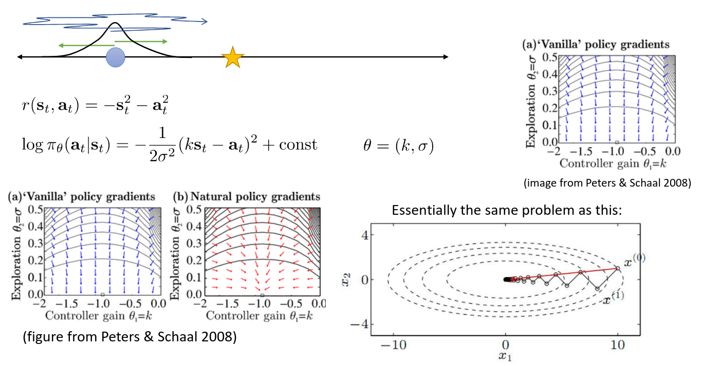
But what's the point of the natural gradient? The idea is that naive gradient ascent experiences problems due to poorly-conditioned functions (see this section from Goodfellow's Deep Learning). See the slide below.

Trust Region Policy Optimization

TRPO is essentially just natural policy gradient.

1. Sample $\{ \tau^{(i)} \}$ from $\pi_{\theta}(\mathbf{a}\mid \mathbf{s})$ (run policy).
2. Evaluate $y_{t}^{(i)}=r(\mathbf{s}_{t}^{(i)},\mathbf{a}_t^{(i)})+\gamma \hat{V}_{\phi}^{\pi}(\mathbf{s}_{t+1}^{(i)})$.
3. Refit $\hat{V}_{\phi}^{\pi}$ to targets $\{ y_{t}^{(i)} \}$, minimizing $\mathcal{L}(\phi)$.
4. Evaluate $\hat{A}_{\text{GAE}}^{\pi}(\mathbf{s}_{t}^{(i)},\mathbf{a}_{t}^{(i)})=\sum_{t'=t}^{\infty}(\gamma\lambda)^{t'-t}\delta_{t'}^{(i)}$.
5. $\theta'\leftarrow\theta+\alpha \mathbf{F}^{-1}\nabla_{\theta}J(\theta)$.

where $\mathbf{F}\approx \frac{1}{N}\sum_{i=1}^{N}\sum_{t=1}^{H}\nabla_{\theta}\log \pi_{\theta}(\mathbf{a}_{t}^{(i)}\mid \mathbf{s}_{t}^{(i)})\nabla_{\theta}\pi_{\theta}(\mathbf{a}_{t}^{(i)}\mid \mathbf{s}_{t}^{(i)})^{\top}$.

Conclusion

• Policy gradient is more productively interpreted as a form of policy iteration.
• PPO with clipping is a heuristic approximation of PPO with KL.
• There are other ways to enforce the constraints
  • Natural gradient!
• TRPO vs PPO? Usually PPO today due to ease of implementation.

Note that TRPO/natural gradient was the precursor to PPO with KL divergence, i.e. PPO is a refinement that offers lower implementation complexity and lower computational complexity.