Lecture 9: Advanced Policy Gradients: Part 1

Return to Policy Gradients

So, why policy gradient? They converge, unlike $Q$ -function methods, and on-policy methods allow Monte Carlo advantage estimators (GAE with $\lambda=1$ ), which provides an unbiased estimator. Thus, policy gradients are stable, reliable methods when sample efficiency is not a concern (samples are cheap to generate).

Let's consider our usual policy gradient algorithm with GAE.

Sample $\{ \tau^{(i)} \}$ from $\pi_{\theta}(\mathbf{a}\mid \mathbf{s})$ (run policy).
Evaluate $y_{i}=r(\mathbf{s}_{t}^{(i)},\mathbf{a}_t^{(i)})+\gamma \hat{V}_{\phi}^{\pi}(\mathbf{s}_{t+1}^{(i)})$ .
Refit $\hat{V}_{\phi}^{\pi}$ to targets $\{ y_{t}^{(i)} \}$ , minimizing $\mathcal{L}(\phi)$ .
Evaluate $\hat{A}_{\text{GAE}}^{\pi}(\mathbf{s}_{t}^{(i)},\mathbf{a}_{t}^{(i)})=\sum_{t'=t}^{\infty}(\gamma\lambda)^{t'-t}\delta_{t'}^{(i)}$ .
Compute $\nabla_{\theta}J(\theta)\approx \sum_{i}\nabla_{\theta}\log \pi_{\theta}(\mathbf{a}_{i}\mid \mathbf{s}_{i})\hat{A}^{\pi}(\mathbf{s}_{t}^{(i)},\mathbf{a}_{t}^{(i)})$ .
Update $\theta\leftarrow\theta+\alpha \nabla_{\theta}J(\theta)$ .

As it is now, it is computationally intractable for practical purposes.

Each iteration takes one gradient step
Each iteration requires generating new samples
It is high variance, and therefore requires large batches and smaller learning rates (in other words, more iterations)

Really, it'd be nice to take multiple gradient steps for every sampling. In other words, repeat steps 5-6 some $K$ times for every execution of steps 1-4. However, this is problematic—the trajectories being used are produced by an old policy, not $\pi_{\theta}$ .

The primary goal of this lecture will be to derive an algorithm that can achieve this goal without issue.

Importance Sampling

Importance sampling is a technique that estimates an expected value under a distribution from which we did not sample on. This is exactly our problem :)

It's described mathematically as follows.

\begin{align*} \mathbb{E}_{x\sim p(x)}[f(x)] &= \int p(x)f(x) \,\mathrm{d}x \\ &= \int \frac{q(x)}{q(x)}p(x)f(x) \,\mathrm{d}x \\ &= \int q(x) \frac{p(x)}{q(x)}f(x) \,\mathrm{d}x \\ &= \mathbb{E}_{x\sim q(x)}\left[ \frac{p(x)}{q(x)}f(x) \right] \end{align*}

Thus, our objective function

J(\theta)=\mathbb{E}_{\tau \sim p_{\theta}(\tau)}[r(\tau)]

may be written using samples from a different policy $\bar{p}$ as

J(\theta)=\mathbb{E}_{\tau \sim \bar{p}(\tau)}\left[ \frac{p_{\theta}(\tau)}{\bar{p}(\tau)}r(\tau) \right]

However, there's one critical issue with this formula. We do not assume knowledge of $p_{\theta}$ , as $p_{\theta}(\tau)=p(\mathbf{s}_{1})\prod_{t=1}^{H}\pi_{\theta}(\mathbf{a}_{t}\mid \mathbf{s}_{t})p(\mathbf{s}_{t+1}\mid \mathbf{s}_{t},\mathbf{a}_{t})$ . In other words, it's dependent on state transition probabilities, which we may not know. However, consider that

\frac{p_{\theta}(\tau)}{\bar{p}(\tau)} = \frac{\cancel{ p(\mathbf{s}_{1}) }\prod_{t=1}^{H} \pi_{\theta}(\mathbf{a}_{t}\mid \mathbf{s}_{t})\cancel{ p(\mathbf{s}_{t+1}\mid \mathbf{s}_{t},\mathbf{a}_{t}) }}{\cancel{ p(\mathbf{s}_{1}) }\prod_{t=1}^{H} \bar{\pi}(\mathbf{a}_{t}\mid \mathbf{s}_{t})\cancel{ p(\mathbf{s}_{t+1}\mid \mathbf{s}_{t},\mathbf{a}_{t}) }} = \prod_{t=1}^{H} \frac{\pi_{\theta}(\mathbf{a}_{t}\mid \mathbf{s}_{t})}{\bar{\pi}(\mathbf{a}_{t}\mid \mathbf{s}_{t})}

This ratio may be computed using only knowledge of our policies!

Let's look at the gradients for a policy gradient algorithm with importance sampling. Define

J(\theta')=\mathbb{E}_{\tau \sim p_{\theta}(\tau)}\left[ \frac{p_{\theta'}(\tau)}{p_{\theta}(\tau)}r(\tau) \right]

Then,

\nabla_{\theta'}J(\theta')=\mathbb{E}_{\tau \sim p_{\theta}(\tau)}\left[ \frac{\nabla_{\theta'}p_{\theta'}(\tau)}{p_{\theta}(\tau)}r(\tau) \right]=\mathbb{E}_{\tau \sim p_{\theta}(\tau)}\left[ \frac{p_{\theta'}(\tau)}{p_{\theta}(\tau)}\nabla_{\theta'}\log p_{\theta'}(\tau)r(\tau) \right]

where we once again use the identity that $p_{\theta}(\tau)\nabla_{\theta}\log p_{\theta}(\tau)=\nabla_{\theta}p_{\theta}(\tau)$ , only for $\theta=\theta'$ here. Note that this similar to the on-policy policy gradient expression, except with an extra term $\frac{p_{\theta'}(\tau)}{p_{\theta}(\tau)}$ to account for the difference in policy.

We can substitute some terms in now (recall from policy gradient) to produce

\nabla_{\theta'}J(\theta') = \mathbb{E}_{\tau \sim p_{\theta}(\tau)}\left[ \left( \prod_{t=1}^{H} \frac{\pi_{\theta'}(\mathbf{a}_{t}\mid \mathbf{s}_{t})}{\pi_{\theta}(\mathbf{a}_{t}\mid \mathbf{s}_{t})} \right)\left( \sum_{t=1}^{H} \nabla_{\theta'}\log \pi_{\theta'}(\mathbf{a}_{t}\mid \mathbf{s}_{t}) \right)\left( \sum_{t=1}^{H} r(\mathbf{s}_{t}, \mathbf{a}_{t}) \right) \right]

which may be rewritten with causality as

\nabla_{\theta'}J(\theta') = \mathbb{E}_{\tau \sim p_{\theta}(\tau)} \left[ \sum_{t=1}^{H} \nabla_{\theta'}\log \pi_{\theta'} (\mathbf{a}_{t}\mid \mathbf{s}_{t}) \underbrace{ \left( \prod_{t'=1}^{t} \frac{\pi_{\theta'}(\mathbf{a}_{t'}\mid \mathbf{s}_{t'})}{\pi_{\theta}(\mathbf{a}_{t'}\mid \mathbf{s}_{t'})} \right) }_{ A } \left( \sum_{t'=t}^{H} r( \mathbf{s}_{t'},\mathbf{a}_{t'}) \underbrace{ \cancel{ \left( \prod_{t''=t}^{t'} \frac{\pi_{\theta'}(\mathbf{a}_{t''}\mid \mathbf{s}_{t''})}{\pi_{\theta}(\mathbf{a}_{t''}\mid \mathbf{s}_{t''})} \right) } }_{ B } \right) \right]

where term $A$ implements causality to ensure future actions don't affect the current weight, and term $B$ represents the probability that this reward $r(\mathbf{s}_{t'},\mathbf{a}_{t'})$ represents the current policy. These are essentially the "weights" assigned to each reward.

info

Term $B$ is typically eliminated for, intuitively, the same motivation as the ideas from the [[Lecture 8#Double $Q$ -Learning|double Q-learning]] section, i.e. maximizing over an old policy is actually more effective. We explore this in more detail next lecture.

We'll focus more on term $A$ for the above reason. It turns out that term $A$ can actually prove very problematic—as a product over such long time intervals, with each term likely $<1$ since the trajectory produced by the old policy is likely to have a greater probability under the old policy compared to the new policy, it will vanish at an exponential rate as $t$ increases.

Now, let's rewrite this expectation in terms of sampling.

\nabla_{\theta'}J(\theta') \approx \frac{1}{N}\sum_{i=1}^{N} \sum_{t=1}^{H} \frac{\pi_{\theta'}(\mathbf{s}_{t}^{(i)},\mathbf{a}_{t}^{(i)})}{\pi_{\theta}(\mathbf{s}_{t}^{(i)},\mathbf{a}_{t}^{(i)})}\nabla_{\theta'}\log \pi_{\theta'}(\mathbf{a}_{t}^{(i)}\mid \mathbf{s}_{t}^{(i)})\hat{A}_{t}^{(i)}

where $\pi_{\theta}(\mathbf{s}_{t}^{(i)},\mathbf{a}_{t}^{(i)})$ denotes the probability of the state-action pair $(\mathbf{s}_{t}^{(i)},\mathbf{a}_{t}^{(i)})$ occurring under the policy $\pi_{\theta}$ , over the entire state-action space. This is known as a state-action marginal distribution, and is essentially the same expression as the previous importance sampling ratio product in expectation.

Subsequently, we can expand the state-action marginal

\nabla_{\theta'}J(\theta') \approx \frac{1}{N}\sum_{i=1}^{N} \sum_{t=1}^{H} \cancel{ \frac{\pi_{\theta'}(\mathbf{s}_{t}^{(i)})}{\pi_{\theta}(\mathbf{s}_{t}^{(i)})} } \cdot\frac{\pi_{\theta'}(\mathbf{a}_{t}^{(i)}\mid\mathbf{s}_{t}^{(i)})}{\pi_{\theta}(\mathbf{a}_{t}^{(i)}\mid\mathbf{s}_{t}^{(i)})}\nabla_{\theta'}\log \pi_{\theta'}(\mathbf{a}_{t}^{(i)}\mid \mathbf{s}_{t}^{(i)})\hat{A}_{t}^{(i)}

and then essentially ignore the relative probabilities of state $\mathbf{s}_{t}^{(i)}$ occurring under the different policies because we assume that $\theta'$ is very similar to $\theta$ , and therefore the state distribution will have shifted very little. In other words, we ignore the importance sampling ratios of the previous steps taken on the trajectory to arrive at this state because we assume the probability of arriving at this state, in expectation, should not change much between policies. Therefore, we only care about the importance sampling ratio of the action probabilities for the current state. We will explore this detail more precisely next lecture. Thus,

\nabla_{\theta'}J(\theta')\approx \frac{1}{N}\sum_{i=1}^{N} \sum_{t=1}^{H} \frac{\pi_{\theta'}(\mathbf{a}_{t}^{(i)}\mid \mathbf{s}_{t}^{(i)})}{\pi_{\theta}(\mathbf{a}_{t}^{(i)}\mid \mathbf{s}_{t}^{(i)})}\nabla_{\theta'}\log \pi_{\theta'}(\mathbf{a}_{t}^{(i)}\mid \mathbf{s}_{t}^{(i)})\hat{A}_{t}^{(i)}

Now, finally, we can reconstruct our multi-step policy gradient algorithm with importance sampling.

Sample $\{ \tau^{(i)} \}$ from $\pi_{\theta}(\mathbf{a}\mid \mathbf{s})$ (run policy).
Evaluate $y_{i}=r(\mathbf{s}_{t}^{(i)},\mathbf{a}_t^{(i)})+\gamma \hat{V}_{\phi}^{\pi}(\mathbf{s}_{t+1}^{(i)})$ .
Refit $\hat{V}_{\phi}^{\pi}$ to targets $\{ y_{t}^{(i)} \}$ , minimizing $\mathcal{L}(\phi)$ .
Evaluate $\hat{A}_{\text{GAE}}^{\pi}(\mathbf{s}_{t}^{(i)},\mathbf{a}_{t}^{(i)})=\sum_{t'=t}^{\infty}(\gamma\lambda)^{t'-t}\delta_{t'}^{(i)}$ .
$\theta'\leftarrow\theta$
6. $\nabla_{\theta'}J(\theta')\approx \frac{1}{N}\sum_{i=1}^{N} \sum_{t=1}^{H} \frac{\pi_{\theta'}(\mathbf{a}_{t}^{(i)}\mid \mathbf{s}_{t}^{(i)})}{\pi_{\theta}(\mathbf{a}_{t}^{(i)}\mid \mathbf{s}_{t}^{(i)})}\nabla_{\theta'}\log \pi_{\theta'}(\mathbf{a}_{t}^{(i)}\mid \mathbf{s}_{t}^{(i)})\hat{A}_{t}^{(i)}$ .
7. $\theta'\leftarrow\theta'+\alpha \nabla_{\theta'}J(\theta')$ .
$\theta\leftarrow\theta'$ .

where the inner loop is repeated some $K$ times.

Practical Importance Sampling

Clipped Importance Weights

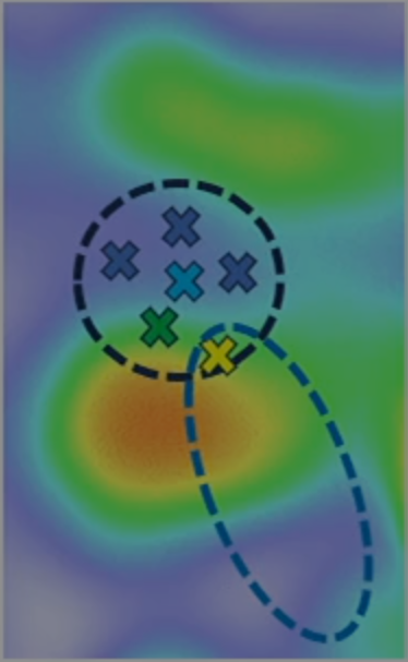
One issue is that, once the importance weights $\frac{\pi_{\theta'}(\mathbf{a}_{t}^{(i)}\mid \mathbf{s}_{t}^{(i)})}{\pi_{\theta}(\mathbf{a}_{t}^{(i)}\mid \mathbf{s}_{t}^{(i)})}$ stray too far from $1.0$ , the estimator is encouraged to over-prioritize good samples and over-penalize bad samples, causing high variance. The below figure shows what might happen.

We can fix this by clipping the importance weights. Let $w(\tau)=\frac{p_{\theta'}(\tau)}{p_{\theta}(\tau)}$ . We clip by defining

w(\tau)=\max \left\{ 1-\epsilon,\min \left\{ 1+\epsilon, \frac{p_{\theta'}(\tau)}{p_{\theta}(\tau)} \right\} \right\}

in other words, $\lVert 1-\frac{p_{\theta}(\tau)}{p_{\theta}(\tau)} \rVert\leq\epsilon$ , which prevents the algorithm from weighting good samples too heavily.

There's one more detail to consider though. Consider a good sample with $w(\tau_{\text{g}})<1+\epsilon$ , and a bad sample with $w(\tau_{\text{b}})\geq 1+\epsilon$ , such that the two samples are similar enough that increasing $w(\tau_{\text{g}})$ will increase $w(\tau_{\text{b}})$ , and vice versa. Notably, the estimator is only ever encouraged to increase $w(\tau)$ (and thus increase the probability of choosing $\tau$ under the new policy $\theta'$ ) for these samples because $w(\tau_{\text{b}})$ will stay constant, but $w(\tau_{\text{g}})$ will increase, based on the clipping. However, this may result in the algorithm making a change that substantially increases the probability of $\tau_{\text{b}}$ under the new policy for only marginal improvements in the probability of $\tau_{\text{g}}$ , because in the perspective of the algorithm with importance weight clipping, this is always an improvement. Thus, the clipping is modified a little bit to be

\begin{align*} J(\theta') &= \mathbb{E}_{\tau \sim p_{\theta}(\tau)}[\min \{ w(\tau)r(\tau),w_{c}(\tau)r(\tau) \}] \\ w(\tau) &= \frac{p_{\theta'}(\tau)}{p_{\theta}(\tau)} \\ w_{c}(\tau) &= \max \left\{ 1-\epsilon,\min \left\{ 1+\epsilon, \frac{p_{\theta'}(\tau)}{p_{\theta}(\tau)} \right\} \right\} \end{align*}

where, essentially, $w(\tau)$ is clipped for good samples, but is not clipped for bad samples. In other words, the bad samples can become arbitrarily bad, but the good samples are always bounded by how good they can be.

Proximal Policy Optimization

Subsequently, we can now implement proximal policy optimization (PPO), or policy gradient with clipped importance sampling.

Sample $\{ \tau^{(i)} \}$ from $\pi_{\theta}(\mathbf{a}\mid \mathbf{s})$ (run policy).
Evaluate $y_{t}^{(i)}=r(\mathbf{s}_{t}^{(i)},\mathbf{a}_t^{(i)})+\gamma \hat{V}_{\phi}^{\pi}(\mathbf{s}_{t+1}^{(i)})$ .
Refit $\hat{V}_{\phi}^{\pi}$ to targets $\{ y_{t}^{(i)} \}$ , minimizing $\mathcal{L}(\phi)$ .
Evaluate $\hat{A}_{\text{GAE}}^{\pi}(\mathbf{s}_{t}^{(i)},\mathbf{a}_{t}^{(i)})=\sum_{t'=t}^{\infty}(\gamma\lambda)^{t'-t}\delta_{t'}^{(i)}$ .
$\theta'\leftarrow\theta$ .
1. $\nabla_{\theta'}J(\theta')\approx \nabla_{\theta'}\mathcal{L}_{\text{CLIP}}(\theta')$
2. $\theta'\leftarrow\theta'+\alpha \nabla_{\theta'}J(\theta')$ .
$\theta\leftarrow\theta'$ .

where we define

\mathcal{L}_{\text{CLIP}}(\theta')=\sum_{i=1}^{N} \sum_{t=1}^{H} \min \left\{ \frac{\pi_{\theta'}(\mathbf{a}_{t}^{(i)}\mid \mathbf{s}_{t}^{(i)})}{\pi_{\theta}(\mathbf{a}_{t}^{(i)}\mid \mathbf{s}_{t})^{(i)}}\hat{A}_{t}^{(i)},\text{clip}\left( \frac{\pi_{\theta'}(\mathbf{a}_{t}^{(i)}\mid \mathbf{s}_{t}^{(i)})}{\pi_{\theta}(\mathbf{a}_{t}^{(i)}\mid \mathbf{s}_{t}^{(i)})},1-\epsilon,1+\epsilon \right)\hat{A}_{t}^{(i)} \right\}

Other Practical Details

Use GAE for $y_{t}^{(i)}$ .
Add $\sum_{i}\sum_{t}\mathcal{H}(\pi_{\theta'}(\cdot \mid \mathbf{s}_{t}^{(i)}))$ to the objective for entropy regularization that encourages exploration (because the agent now tries to maximize entropy as well).