Lecture 12: Variational Inference in RL

Amortized Variational Inference

The problem with variational inference, as mentioned at the end of last lecture, is that there are far too many parameters to tractably train. So, how can we resolve this?

Recall that $q_{i}(z)\approx p(z\mid x_{i})$ . A naive solution might use only one unified $q$ function for all data points, rather than a $q_{i}$ function for each individual data point. This produces a valid lower bound, but... this is probably a terrible lower bound since it's highly unlikely every data point has the same posterior (and if so, your dataset probably isn't good anyways!).

A better solution is to represent all $q_{i}$ with a function $q$ (neural network) such that $q_{i}(z)=q(z\mid x_{i})\approx p(z\mid x_{i})$ , i.e. it produces a distribution over $z$ for each distinct $x_{i}$ . For instance, we could use a function $q_{\phi}(z\mid x)=\mathcal{N}(\mu_{\phi}(x),\sigma_{\phi}(x))$ , where the neural network's parameters are $\phi$ and $\mu_{\phi},\sigma_{\phi}$ are functions that output the posterior's mean and variance given a data point $x$ as input.

Notably, our update step for $q$ doesn't really change; now, we simply update $\phi$ to maximize $\mathcal{L}_{i}(p,q)$ when training on data point $x_{i}$ .

This is known as amortized variational inference, because the difficulty of computing the posterior distribution is "amortized" or distributed across all the data points (rather than determining a posterior for each data point). Our algorithm thus becomes

For each $x_{i}$ /mini-batch
1. Sample $z\sim q_{\phi}(z\mid x_{i})$ and calculate $\nabla_{\theta}\mathcal{L}(p_{\theta}(x_{i}\mid z),q_{\phi}(x_{i}\mid z))\approx \nabla_{\theta}\log p_{\theta}(x_{i}\mid z)$ .
2. $\theta\leftarrow\theta+\alpha \nabla_{\theta}\mathcal{L}$ .
3. $\phi\leftarrow \phi+\alpha \nabla_{\phi}\mathcal{L}$ .

where the loss function for data point $x_{i}$ is

\mathcal{L}_{i}=\mathbb{E}_{z\sim q_{\phi}(z\mid x_{i})}[\log p_{\theta}(x_{i}\mid z)+\log p(z)]+\mathcal{H}(q_{\phi}(z\mid x_{i}))

Now let's define $r(x_{i},z)=\log p_{\theta}(x_{i}\mid z)+\log p(z)$ . Then this becomes

\mathcal{L}_{i}=\mathbb{E}_{z\sim q_{\phi}(z\mid x_{i})}[r(x_{i},z)]+\mathcal{H}(q_{\phi}(z\mid x_{i}))

...hang on, doesn't this look like the expected reward function for an RL problem now? That is, $J(\phi)=\mathbb{E}_{z\sim q_{\phi}(z\mid x_{i})}[r(x_{i},z)]$ is precisely an expected reward function for a "policy" $q_{\phi}$ . This means we can apply RL methods for optimization—in particular, we can just use policy gradient!

Applying policy gradient, we can derive a way to determine $\nabla _{\phi}J(\phi)$ with samples.

\nabla_{\phi} J(\phi)\approx\frac{1}{M}\sum_{j}\nabla_{\phi}\log q_{\phi}(z_{i}\mid x_{i})r(x_{i},z_{i})

and this leads to

\nabla_{\phi}\mathcal{L}_{i}=\nabla_{\phi}J(\phi)+\nabla_{\phi}\mathcal{H}(q_{\phi}(z\mid x_{i}))

so we can now compute our gradient on $\mathcal{L}_{i}$ w.r.t $\phi$ via sampling! (Note that computing $\nabla_{\phi}\mathcal{H}$ is well-known).

But, this gradient has one problem—it's a very high variance gradient. Can we do better?

Reparametrization Trick

Consider that, if $q_{\phi}(z\mid x)=\mathcal{N}(\mu_{\phi}(x),\sigma_{\phi}(x))$ , we can express samples of $z$ as simply $z=\mu_{\phi}(x)+\epsilon\sigma_{\phi}(x)$ where $\epsilon \sim \mathcal{N}(0,1)$ . Notably, this expression is independent of $\phi$ . This allows us to then rewrite

J(\phi)=\mathbb{E}_{\epsilon \sim \mathcal{N}(0,1)}[r(x_{i},\mu_{\phi}(x_{i})+\epsilon\sigma_{\phi}(x_{i}))]

In other words, we have reparametrized the expectation under $\phi$ into an expectation under a constant distribution $\epsilon$ . Then, to estimate $\nabla_{\phi}J(\phi)$ , we can sample $\epsilon \sim \mathcal{N}(0,1)$ instead (usually just one $\epsilon$ ), and then just perform normal backpropagation because $\epsilon$ doesn't depend on $\phi$ .

\nabla_{\phi}J(\phi )\approx \frac{1}{M}\sum_{j}\nabla_{\phi}r(x_{i},\mu_{\phi}(x_{i})+\epsilon_{j}\sigma_{\phi}(x_{i}))

This results in a much lower variance estimator.

Why is this possible here, but not for normal RL? In our normal policy-gradient, $r$ is unknown; it's a function of environment dynamics that we do not assume knowledge of. However, here, we defined and know the expression for $r$ ; therefore, we can compute the gradient of $r$ , and therefore backpropagate gradients through $r$ .

Huh?

Me too. I read this blog (and asked Google/Gemini) to try and understand why. From my limited understanding, it's because we cannot backpropagate through the actual sampling of $z$ from $q_{\phi}(z)$ (due to the stochasticity of sampling). This is problematic because, in standard variational inference, we are trying to compute a gradient w.r.t $\phi$ over an expectation over a distribution parameterized by $\phi$ . We'd like to estimate the expression $\nabla_{\phi}\mathbb{E}_{q_{\phi}(z)}[f(z)]$ via Monte Carlo sampling; to do so, we need to push the gradient operator inside the expectation. However, this is mathematically incorrect—the distribution we are taking the expectation over is parametrized by $\phi$ itself. Thus, a single sample $z\sim q_{\phi}(z)$ does not actually convey any information about the gradient w.r.t $\phi$ , because it carries no information about the distribution $q_{\phi}(z)$ . Without reparametrization, we can use the policy gradient/REINFORCE trick to rewrite the expectation $\nabla_{\phi}\mathbb{E}_{z\sim q_{\phi}(z)}[f(z)]$ as $\mathbb{E}_{z\sim q_{\phi}(z)}[f(z)\nabla_{\phi}\log q_{\phi}(z)]$ ; this is what we did previously. However, this suffers from high variance because it ignores the gradient of $f(z)$ itself. The reparametrization trick helps us rewrite the expression, turning a gradient of an expectation into an expectation of a gradient. By defining $z=g_{\phi}(\epsilon)$ , we can write $\nabla_{\phi}\mathbb{E}_{p(\epsilon)}[f(g_{\phi}(\epsilon))]$ , which allows us to push the gradient operator inside the expectation (since $p(\epsilon)$ is unrelated to $\phi$ ), turning the expression into $\mathbb{E}_{p(\epsilon)}[\nabla_{\phi}f(g_{\phi}(\epsilon))]$ . This gradient now actually uses the gradient of our relevant loss function $f$ , yielding lower variance and consequently faster convergence.

Implementation

We can turn $\mathcal{L}_{i}$ into an equivalent, but more useful, expression for implementation.

\begin{align*} \mathcal{L}_{i} &= \mathbb{E}_{z\sim q_{\phi}(z\mid x_{i})}[\log p_{\theta}(x_{i}\mid z)+\log p(z)]+\mathcal{H}(q_{\phi}(z\mid x_{i})) \\ &= \mathbb{E}_{z\sim q_{\phi}(z\mid x_{i})}[\log p_{\theta}(x_{i}\mid z)]+\mathbb{E}_{z\sim q_{\phi}(z\mid x_{i})}[\log p(z)]+\mathcal{H}(q_{\phi}(z\mid x_{i})) \\ &= \mathbb{E}_{z\sim q_{\phi}(z\mid x_{i})}[\log p_{\theta}(x_{i}\mid z)] - D_{\text{KL}}(q_{\phi}(z\mid x_{i})\parallel p(z)) \\ &= \mathbb{E}_{\epsilon \sim \mathcal{N}(0,1)}[\log p_{\theta}(x_{i}\mid \mu_{\theta}(x_{i})+\epsilon\sigma_{\phi}(x_{i}))]-D_{\text{KL}}(q_{\phi}(z\mid x_{i})\parallel p(z)) \\ &\approx \log p_{\theta}(x_{i}\mid \mu_{\theta}(x_{i})+\epsilon\sigma_{\phi}(x_{i}))-D_{\text{KL}}(q_{\phi}(z\mid x_{i})\parallel p(z)) \end{align*}

As $q_{\phi}(z\mid x_{i})$ and $p(z)$ are both Gaussians, the KL divergence between the two has a nice analytical form. Meanwhile, the gradient of the term on the left may be estimated via Monte Carlo methods, as explained above.

Notably, the resulting architecture is precisely a variational autoencoder (VAE). The encoder network, parametrized by $\phi$ , takes an input $x_{i}$ and produces $\mu_{\phi}(x_{i})$ and $\sigma_{\phi}(x_{i})$ . With the random sampling of some noise $\epsilon \sim \mathcal{N}(0,1)$ , we produce $z=\mu_{\phi}+\epsilon\sigma_{\phi}$ . This $z$ is then fed into the decoder network, parameterized by $\theta$ , to produce $p_{\theta}(x_{i}\mid z)$ . Training is done by backpropagating through the entire computation graph just described for each minibatch of samples. (With the addition of the KL divergence, of course, to the loss function; this may be represented analytically, though, and thus its gradient may be computed without backpropagation).

So what's the intuition behind this? This KL divergence term tries to keep the $q_{\phi}$ closer to the prior $p(z)$ , while the other term tries to ensure the $q_{\phi}$ is good enough such that $p_{\theta}$ may reconstruct (decode) the original $x_{i}$ from the encoded $z=\mu_{\phi}+\epsilon\sigma_{\phi}$ . With the selection of a simple prior, this usually means that the VAE is looking for the simplest $q_{\phi}$ that still does a good job of reconstructing $x_{i}$ (i.e. encodes a simple representation with only the most important information critical to reconstructing $x_{i}$ ).

Reparametrization Trick vs Policy Gradient

Policy gradient

Can handle both discrete and continuous latent variables
High variance

Reparameterization trick

Only continuous latent variables
Simple to implement
Low variance

Generative Models

Variational Autoencoder

First up, the VAE. As aforementioned, it's precisely what we defined above. We have an encoder $q_{\phi}(z\mid x)=\mathcal{N}(\mu_{\phi}(x),\sigma_{\phi}(x))$ and a decoder $p_{\theta}(x\mid z)=\mathcal{N}(\mu_{\theta}(z),\sigma_{\theta}(z))$ . Refer to above for a more detailed explanation on its training.

Note that we may sample (generate $x$ ) from the VAE by first sampling $z\sim p(z)$ and then sampling $x\sim p(x\mid z)$ . Notably, we sample $z$ from the prior $p(z)$ , not the learned posterior $q_{\phi}(z\mid x)$ , as we are generating $x$ and therefore do not have access to $x$ . However, this is okay because our KL divergence term ensured that $q_{\phi}(z\mid x)\approx p(z)$ , and therefore the distribution of $z$ 's seen during training are approximately similar to the distribution of $z$ 's seen at test/inference time.

Representation Learning

We can train a VAE to learn a latent variable $z$ that is a representation of a state $s$ . Then, during training, rather than train our policy to learn off of states as inputs, we use the latent space of the VAE instead of our state space! That is,

Train VAE on states in replay buffer $\mathcal{R}$ .
Run RL using $z$ as the state instead of $s$ .

This is nice because the latent variables are much simpler than the possible states, and the subspaces of the latent space may represent the underlying factors of variation within the state space.

Training this VAE is also a great way to use already existing data, and will likely induce faster convergence for your RL algorithm!

Conditional Models

We can modify our loss function to be

\mathcal{L}_{i}=\mathbb{E}_{z\sim q_{\phi}(z\mid x_{i},y_{i})}[\log p_{\theta}(y_{i}\mid x_{i},z)+\log p(z\mid x_{i})]+\mathcal{H}(q_{\phi}(z\mid x_{i},y_{i}))

this is useful for, say, modeling our policy, i.e. we predict our actions $y_{i}$ given the state $x_{i}$ and the latent variable $z$ , which really represents the different modes of the action distribution (peaks).

This may be used for multimodal imitation learning, since $z$ represents the different modes of the action distribution, i.e. $z$ can be interpreted as a variable of a "latent action suggestion" space.

Relationship to Diffusion and Flow Matching

The below slide summarizes the idea.

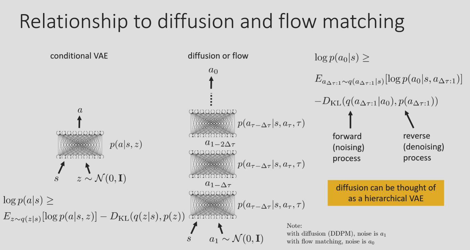
where diffusion is a step-by-step VAE that uses the noising process as its encoder and the denoising process as its prior.

State Space Models

Again, we'll discuss this more when we talk about model-based RL. In essence, though, with a partially-observed RL problem, we use a VAE that almost acts like a recurrent neural network through time steps, i.e. we learn $p(\mathbf{z}_{t+1}\mid \mathbf{z}_{t},\mathbf{a}_{t})$ . The prior is much more complicated, i.e. $p(\mathbf{z})=p(\mathbf{z}_{1})\prod_{t}p(\mathbf{z}_{t+1}\mid \mathbf{z}_{t},a)$ , the decoder is $p_{\theta}(\mathbf{o}\mid \mathbf{z})=\prod_{t}p(\mathbf{o}_{t}\mid \mathbf{z}_{t})$ . and the encoder is $q_{\phi}(\mathbf{z}\mid \mathbf{o})=\prod_{t}q_{\phi}(\mathbf{z}_{t}\mid \mathbf{o}_{1:t})$ . Notably, we have much more freedom of choice with regards to the model for the encoder.

Control as Inference

Imagine trying to train optimal control by modeling human behavior. If we assume humans are perfectly rational, and take actions to maximize some implicit reward function, then this works fine! Unfortunately, humans, and organisms in general, do not exhibit perfect rationality, and therefore do not perform optimal actions.

For example, consider a monkey trying to move an object from one place to another. Typically, the monkey won't follow a perfect, straight-line path; there will be some imperfections. But, crucially, it will allow some certain degree of mistakes or approximation of optimality such that it will still achieve the objective. Thus, the monkey exhibits approximate rationality and includes some stochastic behavior, but in places where it doesn't really matter—the key lesson here is that some mistakes are more important than others!

Thus, when we're modeling, say, human behavior, we shouldn't model some perfect reward maximization algorithm to produce optimal behavior; instead, we should model how humans act approximately optimal, or model the human "intention" of acting optimal.

We can add a binary variable $\mathcal{O}_{t}$ at each time step of a trajectory, where $\mathcal{O}_{t}=1$ denotes a monkey exhibiting the intent of optimal behavior and $\mathcal{O}_{t}=0$ represents the opposite. (In other problems, $\mathcal{O}_{t}$ may take on a wider range of values). And, we will define $p(\mathcal{O}_{t}\mid \mathbf{s}_{t},\mathbf{a}_{t})=\exp(r(\mathbf{s}_{t},\mathbf{a}_{t}))$ , where $r(\mathbf{s}_{t},\mathbf{a}_{t})<0$ so that $p(\mathcal{O}_{t}\mid \mathbf{s}_{t},\mathbf{a}_{t})$ is a valid probability distribution. We will see why this is helpful soon.

Now, consider $p(\tau \mid \mathcal{O}_{1:T})$ , which represents the probability of trajectory $\tau$ given that the monkey is trying to be optimal throughout the entire trajectory.

\begin{align*} p(\tau \mid \mathcal{O}_{1:T}) &= \frac{p(\tau,\mathcal{O}_{1:T})}{p(\mathcal{O}_{1:T})} \\ &\propto p(\tau)\prod \exp(r(\mathbf{s}_{t},\mathbf{a}_{t})) = p(\tau)\exp\left( \sum_{t}r(\mathbf{s}_{t},\mathbf{a}_{t}) \right) \end{align*}

this seems pretty intuitive! As the reward of a trajectory increases, the probability of it occurring under optimal monkey behavior increases too. And, critically, we can see how this probabilistic model can assign nonzero probabilities to potentially suboptimal trajectories that are "close enough" to optimal.

This is important because such a model can help us ignore noise in samples of human or otherwise approximately optimal behavior. It's very applicable to control and planning problems, and, in some sense, can provide an intuitive explanation for the benefits of stochasticity.

Now, what sort of relevant inference problems do we care about?

Computing backward messages $\beta_{t}(\mathbf{s}_{t},\mathbf{a}_{t})=p(\mathcal{O}_{t:T}\mid \mathbf{s}_{t},\mathbf{a}_{t})$ , i.e. "how likely will the monkey continue to be optimal for the rest of the episode given the current state and action?"
Computing the policy $p(\mathbf{a}_{t}\mid \mathbf{s}_{t},\mathcal{O}_{1:T})$ , i.e. "how likely is an action given a state and the assumption that the monkey is optimal over the entire trajectory?"
Computing forward messages $\alpha_{t}(\mathbf{s}_{t})=p(\mathbf{s}_{t}\mid \mathcal{O}_{1:t-1})$ , i.e. "how likely is state $\mathbf{s}_{t}$ given the assumption that the monkey was optimal over all previous steps?"

The key idea here is that backward messages will help us compute a policy, while forward messages will help us figure out the state the monkey ends up in.

Backward Messages

Note first that we know $p(\mathcal{O}_{t}\mid \mathbf{s}_{t},\mathbf{a}_{t})\propto \exp(r(\mathbf{s}_{t},\mathbf{a}_{t}))$ . So, we'd like to compute a recursive formula backwards through time, using the last time step as our base case.

\begin{align*} \beta_{t}(\mathbf{s}_{t},\mathbf{a}_{t}) &= p(\mathcal{O}_{t:T}\mid \mathbf{s}_{t},\mathbf{a}_{t}) \\ &= \int p(\mathcal{O}_{t:T},\mathbf{s}_{t+1}\mid \mathbf{s}_{t},\mathbf{a}_{t}) \,\mathrm{d}\mathbf{s}_{t+1} \\ &= \int p(\mathcal{O}_{t+1:T}\mid \mathbf{s}_{t+1})p(\mathbf{s}_{t+1}\mid \mathbf{s}_{t},\mathbf{a}_{t})p(\mathcal{O}_{t}\mid \mathbf{s}_{t},\mathbf{a}_{t}) \,\mathrm{d}\mathbf{s}_{t+1} \\ p(\mathcal{O}_{t+1:T}\mid \mathbf{s}_{t+1}) &= \int \underbrace{ p(\mathcal{O}_{t+1:T}\mid \mathbf{s}_{t+1},\mathbf{a}_{t+1}) }_{ \beta_{t}(\mathbf{s}_{t+1},\mathbf{a}_{t+1}) }p(\mathbf{a}_{t+1}\mid \mathbf{s}_{t+1}) \,\mathrm{d}\mathbf{a}_{t+1} \longrightarrow\beta_{t}(\mathbf{s}_{t}) \end{align*}

Note the use of the Markov property in the second step. Also, note that $p(\mathbf{a}_{t+1}\mid \mathbf{s}_{t+1})$ is a prior for our actions, and represents the monkey's actions under zero optimality conditions—this can essentially be assumed to be a uniform distribution and thus ignored, and we will formalize why soon. The above derivation allows us to write

\begin{align*} \beta_{t}(\mathbf{s}_{t},\mathbf{a}_{t}) &= p(\mathcal{O}_{t}\mid \mathbf{s}_{t},\mathbf{a}_{t})\mathbb{E}_{\mathbf{s}_{t+1}\sim p(\mathbf{s}_{t+1}\mid \mathbf{s}_{t},\mathbf{a}_{t})}[\beta_{t+1}(\mathbf{s}_{t+1})] \\ \beta_{t}(\mathbf{s}_{t}) &= \mathbb{E}_{\mathbf{a}_{t}\sim p(\mathbf{a}_{t}\mid \mathbf{s}_{t})}[\beta_{t}(\mathbf{s}_{t},\mathbf{a}_{t})] \end{align*}

and we can iterate from $t=T-1$ to $t=1$ to compute all $\beta_{t}$ values.

Now, let's define

\begin{align*} V_{t}(\mathbf{s}_{t}) &= \log\beta_{t}(\mathbf{s}_{t}) \\ Q_{t}(\mathbf{s}_{t},\mathbf{a}_{t}) &= \log\beta_{t}(\mathbf{s}_{t},\mathbf{a}_{t}) \end{align*}

$V_{t}$ has recursive definition

\begin{align*} V_{t}(\mathbf{s}_{t}) &= \log \int \exp(Q_{t}(\mathbf{s}_{t},\mathbf{a}_{t})) \,\mathrm{d}\mathbf{a}_{t} \end{align*}

We will call $V_{t}$ a soft max.

warning

This is not the same thing as a softmax!!

Why is $V_{t}$ called a soft max? Because $\int \exp$ is dominated by large $Q_{t}(\mathbf{s}_{t},\mathbf{a}_{t})$ , and thus this is a continuous function that approximates the maximum value of $Q_{t}$ . Formally,

\lim_{ Q_{t} \to \infty } V_{t}(\mathbf{s}_{t})=\max _{\mathbf{a}_{t}}Q_{t}(\mathbf{s}_{t},\mathbf{a}_{t})

Meanwhile, $Q_{t}$ has the following recursive definition

Q_{t}(\mathbf{s}_{t},\mathbf{a}_{t}) = r(\mathbf{s}_{t},\mathbf{a}_{t})+\log \mathbb{E}[\exp(V_{t+1}(\mathbf{s}_{t+1}))]

Deterministic Transitions

If state transitions are deterministic, the recursive formula has the form

Q_{t}(\mathbf{s}_{t},\mathbf{a}_{t})=r(\mathbf{s}_{t},\mathbf{a}_{t})+V_{t+1}(\mathbf{s}_{t+1})

which looks exactly like our usual $Q$ -function Bellman update equation, in fact!

Now, with deterministic transitions, if we just throw these functions into value iteration, we get essentially the same thing, except now with our "soft max" function replacing the usual "hard max." But, without deterministic transitions, there's now also a "soft max" function over the possible state transitions; in other words, this encourages excessive optimism, in which the algorithm favors states that may lead to potentially higher-value states, but may also have fairly high probability of low-value states. (Since it takes the expected value of the soft max over the possible next states!). This is pretty bad... but we'll come back to this in future lectures.

Action Prior

Let's now return to the action prior $p(\mathbf{a}_{t}\mid \mathbf{s}_{t})$ . Previously, we just assumed that it was a uniform distribution, but this may not always be the case. (In our monkey example, the monkey might prefer small movement actions because it's lazy). If it isn't uniform, then our recursive definitions change a bit.

\begin{align*} V(\mathbf{s}_{t}) &= \log \int \exp(Q(\mathbf{s}_{t},\mathbf{a}_{t})+\log p(\mathbf{a}_{t}\mid \mathbf{s}_{t})) \,\mathrm{d}\mathbf{a}_{t} \\ Q(\mathbf{s}_{t},\mathbf{a}_{t}) &= r(\mathbf{s}_{t},\mathbf{a}_{t})+\log \mathbb{E}[\exp(V(\mathbf{s}_{t+1}))] \end{align*}

Or, we could simply define a new $Q$ function

\begin{align*} \tilde{Q}(\mathbf{s}_{t},\mathbf{a}_{t}) &= r(\mathbf{s}_{t},\mathbf{a}_{t}) + p(\mathbf{a}_{t}\mid \mathbf{s}_{t})+ \log \mathbb{E}[\exp(V(\mathbf{s}_{t+1}))] \end{align*}

and define $V(\mathbf{s}_{t})$ as

V(\mathbf{s}_{t})=\log \int \exp(\tilde{Q}(\mathbf{s}_{t},\mathbf{a}_{t})) \,\mathrm{d}\mathbf{a}_{t}

In other words, we can treat the action prior as simply modifying the reward function to be $\tilde{r}(\mathbf{s}_{t},\mathbf{a}_{t})=r(\mathbf{s}_{t},\mathbf{a}_{t})+p(\mathbf{a}_{t}\mid \mathbf{s}_{t})$ ! And, hopefully, this should intuitively make sense; a monkey that is lazy in his action prior would, in its perspective, be receiving higher rewards for lazier actions. Now, this mathematical basis actually gives us reason to assume the action prior is simply uniform henceforth; even if it isn't, we can simply modify the reward function to express it.

Policy Computation

Now, we can finally compute our policy $p(\mathbf{a}_{t}\mid \mathbf{s}_{t},\mathcal{O}_{1:T})$ using our backward messages.

\begin{align*} p(\mathbf{a}_{t}\mid \mathbf{s}_{t},\mathcal{O}_{1:T}) &= \pi(\mathbf{a}_{t}\mid \mathbf{s}_{t}) && (1) \\ &= p(\mathbf{a}_{t}\mid \mathbf{s}_{t},\mathcal{O}_{t:T}) && (2) \\ &= \frac{p(\mathbf{a}_{t},\mathbf{s}_{t}\mid\mathcal{O}_{t:T})}{p(\mathbf{s}_{t}\mid \mathcal{O}_{t:T})} && (3) \\ &= \frac{p(\mathcal{O}_{t:T}\mid \mathbf{a}_{t},\mathbf{s}_{t})p(\mathbf{a}_{t},\mathbf{s}_{t})/p(\mathcal{O}_{t:T})}{p(\mathbf{s}_{t},\mathcal{O}_{t:T})/p(\mathcal{O}_{t:T})} && (4) \\ &= \frac{p(\mathcal{O}_{t:T}\mid \mathbf{a}_{t},\mathbf{s}_{t})}{p(\mathcal{O}_{t:T}\mid \mathbf{s}_{t})}\cdot \frac{p(\mathbf{a}_{t},\mathbf{s}_{t})}{p(\mathbf{s}_{t})} && (5) \\ \end{align*}

where the steps are

Definition
Due to the Markov property, $\mathbf{s}_{t}$ captures all that is needed for the previous states; therefore, only the future optimality variables are needed.
Law of Conditional Probability
Bayes' Rule + Law of Conditional Probability
Law of Conditional Probability

The final formula is notably the same as

\pi(\mathbf{a}_{t}\mid \mathbf{s}_{t}) = \frac{\beta_{t}(\mathbf{s}_{t},\mathbf{a}_{t})}{\beta_{t}(\mathbf{s}_{t})}\cancel{ p(\mathbf{a}_{t}\mid \mathbf{s}_{t}) }

where the action prior doesn't matter for the reasons given above. Thus, we have a formula for our policy in terms of our backward messages! But what does this mean? Well, if we replace $\beta_{t}$ here with $V_{t}$ and $Q_{t}$ , we find that

\pi(\mathbf{a}_{t}\mid \mathbf{s}_{t}) = \exp(Q_{t}(\mathbf{s}_{t},\mathbf{a}_{t})-V_{t}(\mathbf{s}_{t}))=\exp(A_{t}(\mathbf{s}_{t},\mathbf{a}_{t}))

Intuitively, this formula says that our policy is just more likely to take the actions that provide higher advantages. (This is effectively analogous to Boltzmann exploration, which was briefly mentioned towards the end of Lecture 7).

Temperature

Larger reward functions result in sharper policies, so oftentimes a temperature constant $\alpha$ is applied, $\pi(\mathbf{a}_{t}\mid \mathbf{s}_{t})=\exp\left( \frac{1}{\alpha}A_{t}(\mathbf{s}_{t},\mathbf{a}_{t}) \right)$ . As temperature decreases, the soft max approaches the hard max function, and the policy approaches a greedy policy.

Forward Messages

We won't discuss the math in detail, but the whole idea and simplification is very similar to the derivation of backward messages. The key point is, though, is that once we have derived the forward messages recursive formula (allowing us to compute the forward messages across an entire trajectory), we can then compute the probability of any state along an optimal trajectory. In fact,

p(\mathbf{s}_{t}\mid \mathcal{O}_{1:T}) \propto \alpha_{t}(\mathbf{s}_{t})\beta_{t}(\mathbf{s}_{t})

and, one may note

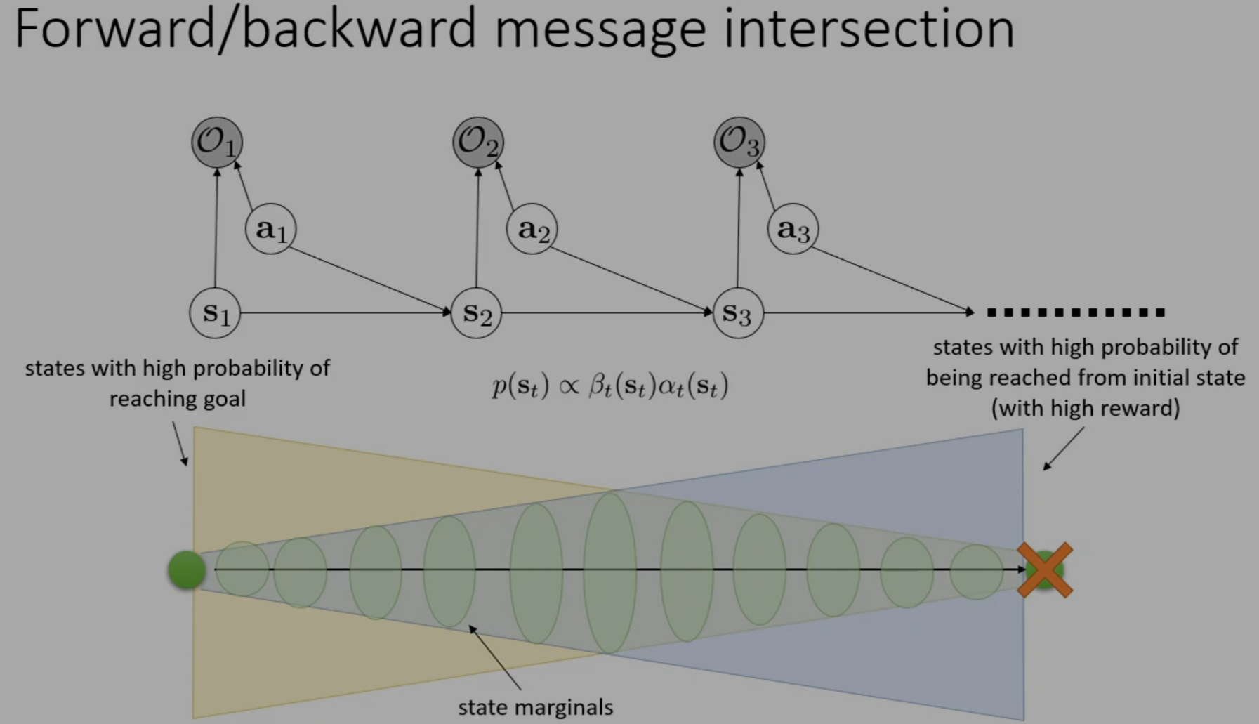
In other words, there is more variability in the middle of the trajectory, and less towards the start and the end of the trajectory. Perhaps intuitive, but now we've formalized this idea :)