Lecture 13: Control as Variational Inference

Theory

Recall that our "control as inference" derivation from Lecture 12 used the following value functions.

recall that, with stochastic environment dynamics, the second term of the $Q$-function expression encourages excessive optimism regarding states with very large rewards/values, even if they occur with very small state transition probabilities. We'd like to eliminate this excessive optimism.

Let's first take a step back and consider: why does this occur in the first place?

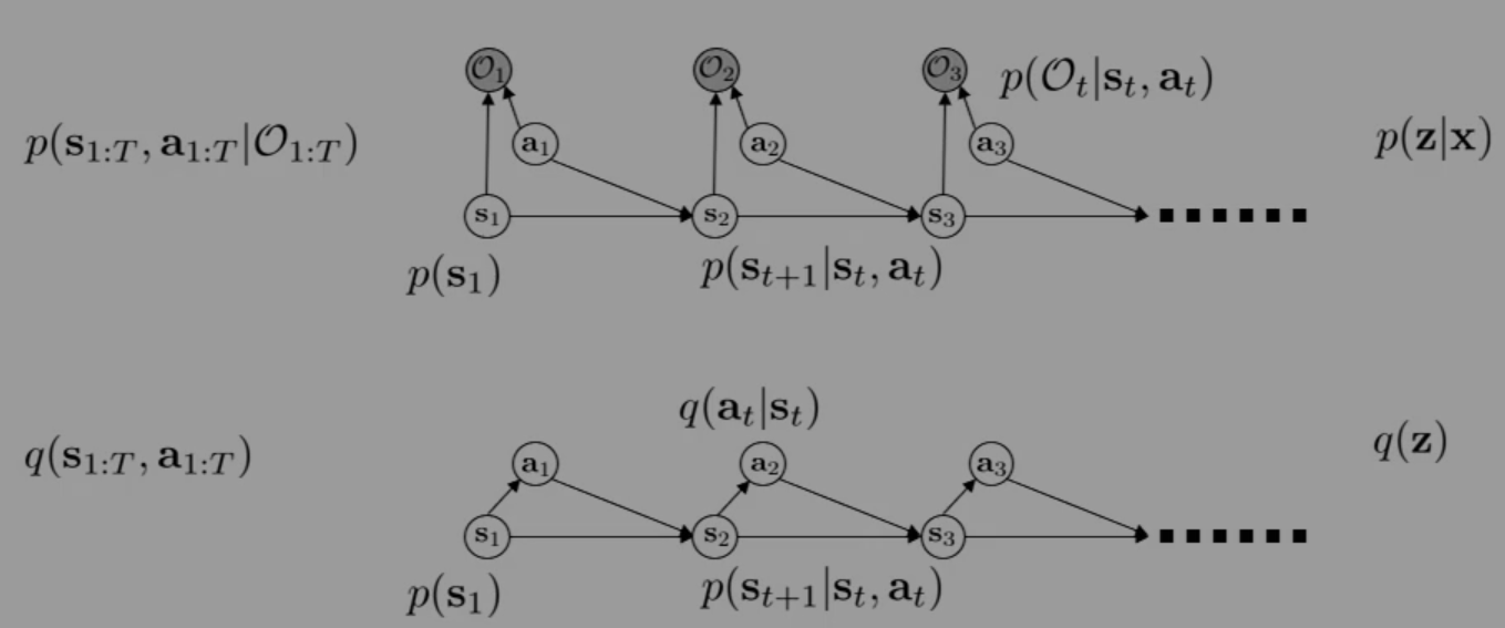
Our inference problem is $p(\mathbf{s}_{1:T},\mathbf{a}_{1:T}\mid \mathcal{O}_{1:T})$, i.e. what is the probability of the trajectory $\tau$ given that the monkey is being optimal? Through marginalization over the time steps $t$ and conditioning on the state $\mathbf{s}_{t}$, we produce the policy $p(\mathbf{a}_{t}\mid \mathbf{s}_{t},\mathcal{O}_{1:T})$, i.e. what is the probability of the action $\mathbf{a}_{t}$ being chosen in state $\mathbf{s}_{t}$ given the optimality of the monkey? However, we may note that $\mathcal{O}_{t}$ is really just an indicator (evidence) of whether or not $\mathbf{a}_{t}$ was high reward or not; thus, this is really asking, "given that you obtained high reward, what was your action probability?" This, intuitively, is a good question to ask—after understanding that we obtained a high reward, we'd like to maximize our action probability for this high reward.

However, when performing inference over the computational graph, the action probabilities are not the only factors; critically, the state transition probabilities are involved too. In fact, we can similarly marginalize over $t$ and condition to produce $p(\mathbf{s}_{t+1}\mid \mathbf{s}_{t},\mathbf{a}_{t},\mathcal{O}_{1:T})\neq p(\mathbf{s}_{t+1}\mid \mathbf{s}_{t},\mathbf{a}_{t})$. That is, "given that you obtained high reward, what was your transition probability?" And this is a bad question to ask! This is like, say, training our model to make a decision on whether or not to buy a lottery ticket after they already observed winning the lottery ticket in the future. However, just because it won this time does not mean that buying a lottery ticket is a good action in general—in essence, the model is learning action optimality from the fact that it "lucked out" from hitting rare state transition probabilities, and believes it can optimize this state transition probability to always happen.

In short, we'd like to phrase the question as "given that you obtained high reward, what was your action probability, given that your transition probability did not change?" More generally, we'd like to find a way to tell the model to maximize the probability of success without changing the environment dynamics. Or, mathematically, we'd like to find another distribution $q(\mathbf{s}_{1:T},\mathbf{a}_{1:T})$ that is close to the posterior $p(\mathbf{s}_{1:T},\mathbf{a}_{1:T}\mid \mathcal{O}_{1:T})$ but has static dynamics $p(\mathbf{s}_{t+1}\mid \mathbf{s}_{t},\mathbf{a}_{t})$ (i.e. the model should not believe it is capable of maximizing state transition probabilities like action probabilities).

Well, we can actually apply variational inference to this problem! Let our observed variables be $\mathbf{x}=\mathcal{O}_{1:T}$ and our latent variables be $\mathbf{z}=(\mathbf{s}_{1:T},\mathbf{a}_{1:T})$. We'd like to find a $q(\mathbf{z})$ that approximates $p(\mathbf{z}\mid \mathbf{x})$; in particular, we will choose to define

Notably, it's very unusual to include $p(\mathbf{s}_{1})$ and $p(\mathbf{s}_{t+1}\mid \mathbf{s}_{t},\mathbf{a}_{t})$ in the definition of $q$, as, in variational inference, it's typically desirable to make $q$ a simple distribution (for a tractable approximation), and we have no guarantees about the simplicity of those distributions derived from the computational graph. We will immediately see why this is useful, though (induces a lot of cancellation below).

Then, according to the ELBO (evidence lower bound)

For the last step, recall that we defined $p(\mathcal{O}_{t}\mid \mathbf{s}_{t},\mathbf{a}_{t})=\exp(r(\mathbf{s}_{t},\mathbf{a}_{t}))$ last lecture. This allows us to subsequently conclude that

This looks pretty similar to what we've seen before; in fact, it's just our regular RL policy gradient objective plus the entropy of the action distribution! Crucially, though, the only thing within the expectation that is not fixed relative to $q$ (since the expectation is computed over $q$) is the action probabilities! Our choice to hardcode the environment dynamics $p(\mathbf{s}_{t})$ and $p(\mathbf{s}_{t+1}\mid \mathbf{s}_{t},\mathbf{a}_{t})$ into $q(\tau)$ cancels with the existing probabilities in $p(\tau,\mathcal{O}_{1:T})$. Thus, our model won't try and modify our state transition probabilities to maximize $p(\mathcal{O}_{1:T})$; it's forced to optimize only $q(\mathbf{a}_{t}\mid \mathbf{s}_{t})$, which is the only aspect the model actually controls.

Just one final note to close this off: we still need to solve for $q(\mathbf{a}_{t}\mid \mathbf{s}_{t})$ for all $t$. We can recurse backwards, like we did for backwards messages. We first compute the base case

and then, with many steps of mathematical derivation, we can derive

where $Q(\mathbf{s}_{t},\mathbf{a}_{t})=r(\mathbf{s}_{t},\mathbf{a}_{t})+\mathbb{E}[V_{t+1}(\mathbf{s}_{t+1})]$. Notably, it is now a regular Bellman backup equation; it's no longer optimistic.

And thus, we can compute our value functions backwards through time with our recursive expressions. For $t=T-1$ to $1$,

and we now have a soft value iteration algorithm:

1. Set $Q(\mathbf{s},\mathbf{a})\leftarrow r(\mathbf{s},\mathbf{a})+\mathbb{E}[V(\mathbf{s}')]$.
2. Set $V(\mathbf{s})\leftarrow\text{soft max}_{\mathbf{a}}\ Q(\mathbf{s},\mathbf{a})$.

Various modifications like discounting and temperature may also be added.

Maximum Entropy RL Algorithms

$Q$-Learning with soft optimality

Standard $Q$-learning uses the hard max over the $Q$ values to determine the value function, i.e. $V(\mathbf{s}')=\max_{\mathbf{a}'}Q_{\phi}(\mathbf{s}',\mathbf{a}')$. For soft $Q$-learning, we just change the hard max to soft max. Ultimately, this not a very popular algorithm because, for small action spaces, the hard max works just fine.

Policy Gradient with soft optimality

Recall that the control with variational inference strategy ended up with a policy gradient objective with an added action entropy term. The modification to policy gradient is precisely the same, just define $J(\theta)=\sum_{t}\mathbb{E}_{(\mathbf{s}_{t},\mathbf{a}_{t})\sim \pi_{\theta}}[r(\mathbf{s}_{t},\mathbf{a}_{t})+\mathcal{H}(\pi_{\theta}(\mathbf{a}_{t}\mid \mathbf{s}_{t}))]$. This is very commonly applied, because it's simple to add (entropy usually has a closed form expression for most policy classes) and policy gradient often collapses to a deterministic, non-exploratory policy too soon during training.

Soft Actor-Critic

This is the most well-known application of soft optimality. We modify two things:

where you may recall that the $y_{i}$ are the target values used to train the critic $\hat{Q}_{\phi}^{\pi}$. Note that, conventionally, the entropy for the $Q$-function is usually estimated, i.e.

Also, it's very common to add a "temperature" $\beta$ as a coefficient to the entropy terms.

Inverse Reinforcement Learning

In standard imitation learning, e.g. behavioral cloning, the model attempts to copy the actions the expert takes, without any reasoning about the action outcomes. In contrast, humans, when learning, attempt to copy the intent of the expert, and consequently may take very different actions due to their reasoning about the expert's intent. Thus, it's potentially very useful to learn reward functions from demonstrations, rather than have the developer define a reward function for the model to optimize.

Our previous soft optimality or control as inference framework is very helpful for this. Let's use the same probabilistic model with the same optimality variable; but now, instead of learning a policy based on a reward function, we will attempt to learn a reward function given trajectories sampled from a soft-optimal policy. In other words, we have

and consequently

Note that there's a hidden denominator involved with the expression as well that's not shown in the proportionality equation. In particular, the denominator is $Z$, the partition function $Z=\int p(\tau)\exp(r_{\psi}(\tau)) \,\mathrm{d}\tau$.

Maximum likelihood learning tells us that the optimal $\psi$ is simply

Also, we may note that, when taking the gradient of $p(\tau \mid \mathcal{O}_{1:T},\psi)$ w.r.t $\psi$, $p(\tau)$ is irrelevant since it represents the environment dynamics and is thus independent of the reward parameters. Therefore, we're really considering

where $\log Z$ shows up due to the hidden $Z$ denominator, as aforementioned.

Notably, the gradient is zero when $\pi^{*}(\tau)$, the policy of our expert that we estimate with samples, is equivalent to $p(\tau \mid \mathcal{O}_{1:T},\psi)$, the soft optimal policy produced by following our current estimated reward function.

Additionally, because the partition function $Z$ integrates over all possible trajectories, it is of course intractable to compute directly. Therefore, we must estimate it instead—we can use variational inference, which dictates that we should train a maximum entropy RL agent to approximate the intractable optimal policy for the current reward function $r_{\psi}$. Only then may we sample from this policy to produce trajectories $\tau$ for the second term $\mathbb{E}_{\tau \sim p(\tau \mid \mathcal{O}_{1:T},\psi)}[\nabla_{\psi}r_{\psi}(\tau)]$.