Lecture 14: RL with Sequences and LLMs

Reward Learning and Inverse RL

Recall the idea of inverse reinforcement learning (IRL): learning a model of the reward function demonstrated through some samples from an "expert" actor. This is in contrast to behavioral cloning in imitation learning, which simply seeks to mimic the behavior of the expert, and therefore expresses limited generalization to unseen states that require similar reasoning. (There are also other advantages of IRL, such as a lack of the compounding error from distributional shift that behavioral cloning typically encounters).

When we attempt to apply inverse RL to our previous soft optimality framework, we attempt to learn the reward model, provided we have sample trajectories from a soft-optimal policy. We use the equation

p(\mathcal{O}_{t}\mid \mathbf{s}_{t},\mathbf{a}_{t},\psi)=\exp(r_{\psi}(\mathbf{s}_{t},\mathbf{a}_{t}))

and use maximum likelihood estimation to find that

\hat{\psi}=\underset{\psi}{\arg\max}\ \frac{1}{N}\sum_{i=1}^{N} \log p(\tau_{i}\mid \mathcal{O}_{1:T},\psi)=\underset{\psi}{\arg\max}\ \frac{1}{N}\sum_{i=1}^{N} r_{\psi}(\tau_{i})-\log Z

where $Z$ is the inverse RL partition function, and is equivalent to

Z=\int p(\tau)\exp r_{\psi}(\tau) \,\mathrm{d}\tau

Note that $Z$ functions as a "normalizer" for $\psi$ in order to produce a probability distribution, considering that the rewards themselves are unnormalized. Taking the gradient of our loss function, we find that

\begin{align*} \nabla_{\psi}\mathcal{L} &= \frac{1}{N}\sum_{i=1}^{N} \nabla_{\psi}r_{\psi}(\tau_{i})-\underbrace{ \frac{1}{Z}\int p(\tau)\exp(r_{\psi}(\tau)) }_{ p(\tau \mid \mathcal{O_{1:T},\psi}) }\nabla_{\psi}r_{\psi}(\tau) \,\mathrm{d}\tau \\ &= \mathbb{E}_{\tau \sim \pi^{*}(\tau)}[\nabla_{\psi}r_{\psi}(\tau_{i})]-\mathbb{E}_{\tau \sim p(\tau \mid \mathcal{O}_{1:T},\psi)}[\nabla_{\psi}r_{\psi}(\tau)] \end{align*}

In words, these expectations are over trajectories produced by the...

\nabla_{\psi}\mathcal{L} = \underbrace{ \mathbb{E}_{\tau \sim \pi^{*}(\tau)}[\nabla_{\psi}r_{\psi}(\tau_{i})] }_{ \text{expert policy} }-\underbrace{ \mathbb{E}_{\tau \sim p(\tau \mid \mathcal{O}_{1:T},\psi)}[\nabla_{\psi}r_{\psi}(\tau)] }_{ \text{soft optimal policy w/ current reward} }

For estimating that second expectation, i.e. the expectation over trajectories from our soft optimal policy, we can apply any maximum-entropy RL algorithm (see Lecture 13). Thus, we can just do

\nabla_{\psi}\mathcal{L}\approx\underbrace{ \frac{1}{N}\sum_{i=1}^{N} \nabla_{\psi}r_{\psi}(\tau_{i}) }_{ \text{expert samples} } -\underbrace{ \frac{1}{M}\sum_{j=1}^{M} \nabla_{\psi}r_{\psi}(\tau_{j}) }_{ \text{policy samples} }

Unfortunately, this method is computationally expensive. (Why? We effectively have two nested loops of gradient ascent; for every step we take on $\psi$ , we have to run an entire maximum-entropy RL algorithm to relearn our soft optimal policy). So, can we do better?

Taking ideas from generalized policy iteration, we can be "lazy" with our relearning of our soft optimal policy; instead of learning an estimate of $p(\mathbf{a}_{t} \mid \mathbf{s}_{t,}\mathcal{O}_{1:T},\psi)$ until convergence every time we update $r_{\psi}$ , we only make a marginal update (take a few policy gradient/max-entropy algorithm steps on our policy $p$ ) that brings us closer to the soft optimal policy for our new reward function. Sadly, this is not valid and produces a biased estimate—our second expectation is now being performed over samples taken from a non-optimal policy for our reward function...

...wait. Training on samples taken from a trajectory distribution produced by another policy? Isn't that just off-policy learning? So we can just use importance sampling to correct our algorithm!

\begin{align*} \nabla_{\psi}\mathcal{L} &\approx \frac{1}{N}\sum_{i=1}^{N} \nabla_{\psi}r_{\psi}(\tau_{i}) - \frac{1}{\sum_{j}w_{j}}\sum_{j=1}^{M} w_{j}\nabla_{\psi}r_{\psi}(\tau_{j}) \end{align*}

where we define

\begin{align*} w_{j} &= \frac{p(\tau)\exp(r_{\psi}(\tau_{j}))}{\pi(\tau_{j})}=\frac{p(\mathbf{s}_{1})\prod_{t}p(\mathbf{s}_{t+1}\mid \mathbf{s}_{t},\mathbf{a}_{t})\exp(r_{\psi}(\mathbf{s}_{t},\mathbf{a}_{t}))}{p(\mathbf{s}_{1} )\prod_{t}p(\mathbf{s}_{t+1}\mid \mathbf{s}_{t},\mathbf{a}_{t})\pi(\mathbf{a}_{t}\mid \mathbf{s}_{t})} \\ &= \frac{\exp\left( \sum_{t}r_{\psi}(\mathbf{s}_{t},\mathbf{a}_{t}) \right)}{\prod_{t}\pi(\mathbf{a}_{t}\mid \mathbf{s}_{t})} \end{align*}

intuitively, this just weights samples according to their reward, computed by the current reward function, relative to the probability of the sample occurring under the non-optimal policy. In other words, reweighting the samples to more heavily favor those that the optimal policy of the current reward function would have been more likely to take.

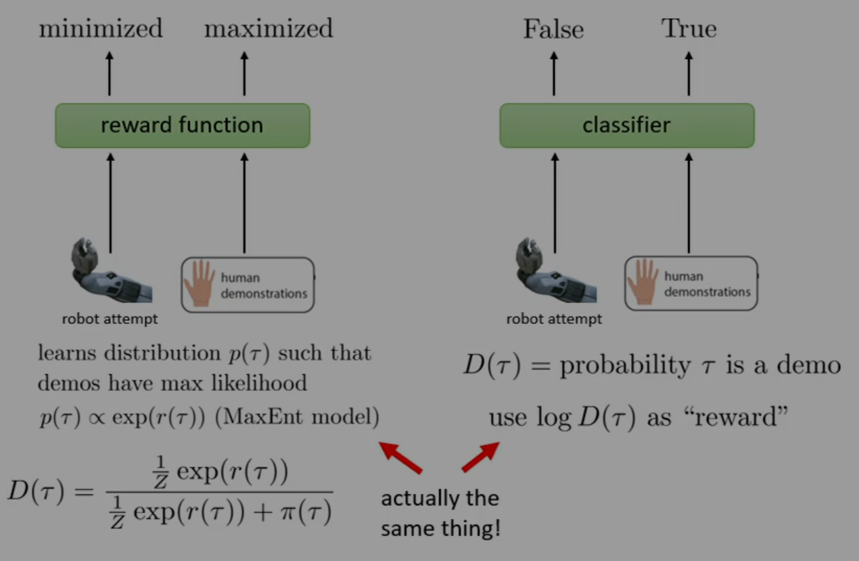
One may interpret this training procedure as a two-player adversarial game. There is a discriminator, $\psi$ , that attempts to increase the likelihood of samples from the expert demonstrations (positive first expectation $\mathbb{E}_{\tau \sim \pi^{*}(\tau)}$ encourages gradient ascent on/maximization of rewards from the expert trajectories), and simultaneously decreases the likelihood of samples from the policy $\theta$ (negative second expectation $-\mathbb{E}_{\tau \sim p(\mathbf{a}_{t}\mid \mathbf{s}_{t},\mathcal{O}_{1:T},\psi)}$ encourages gradient descent on/minimization of rewards from policy trajectories). Meanwhile, the generator $\theta$ is continuously improved to make it harder for $\psi$ to distinguish between samples from the expert and samples from $\theta$ . In this way, we continually improve our reward function and policy in a competing manner, until convergence at an equilibrium where the $\pi^{*}=p(\mathbf{a}_{t}\mid \mathbf{s}_{t},\mathcal{O}_{1:T},\psi)$ , i.e. the policy is encouraged to imitate the expert.

Such game-like models are known as generative adversarial networks (GANs). A discriminator model is trained to distinguish between samples from a dataset and samples from a generator model, while the generator model is optimized to fool the discriminator.

So, let's go back and approach this question from the beginning, but with the intent of designing a GAN for our problem. We still have a policy as our generator model, but instead of a reward model, we'll use a binary discriminator.

\psi\leftarrow \underset{\psi}{\arg\max}\ \mathbb{E}_{\tau \sim p^{*}}[\log D_{\psi}(\tau)]+\mathbb{E}_{\tau \sim \pi_{\theta}}[\log(1-D_{\psi}(\tau))]

and our policy gradient is

\nabla_{\theta}\mathcal{L}\approx \frac{1}{M}\sum_{j=1}^{M} \nabla_{\theta}\log \pi_{\theta}(\tau_{j})\log D_{\psi}(\tau_{j})

This is much simpler to implement than our inverse RL algorithm. However, at the end of training, since the policy is essentially identical to the expert demonstrations, the discriminator will learn to simply output $0.5$ probability on every input; that is, the discriminator knows nothing at convergence! Moreover, it's generally not possible to reoptimize the reward function $D$ .

In short, though, we have the following comparison.

RL and LLMs: The Basics

Important questions for applying RL to LLMs:

What is the (PO)MDP, i.e. (partially observed) Markov decision process?
What is the reward function?
What algorithm do we use?

First, we discuss a short anatomy of LLM training.

Pre-training: Supervised training on a large corpus of data, gives LLM knowledge.
Post-training: Tells LLM how to use its knowledge.
- Supervised fine-tuning (SFT) (instruction tuning, basically imitation learning) on a smaller, high-quality dataset that demonstrates what you want the LLM to do (e.g. be a helpful model).
- RL fine-tuning (e.g. reinforcement learning from human feedback/RLHF).

Instruction tuning was the initial LLM post-training methodology. However, it's labor-intensive to collect an SFT dataset, especially for skilled tasks like programming. Reinforcement learning offers a more tractable solution.

There are two main approaches to RL post-training.

Training an LLM to appeal to human preferences. This can be dangerous, though, if preferences do not actually reflect what's desirable (e.g. LLM removes all test cases to pass all unit tests).
Training an LLM to be correct. (a.k.a. RL from verifiers). Typically, "thinking mode" is a product of this. This is difficult to check objectively, however.

So how do we define our MDP for an LLM? There are a couple methods.

Define $p(\mathbf{a}\mid \mathbf{s})$ where $\mathbf{a}$ is the response and $\mathbf{s}$ is the prompt, i.e. creating a one-step MDP.
Define $\pi_{\theta}(\mathbf{a}_{t}\mid \mathbf{s}_{t})$ for all tokens $t$ in the response, where $\mathbf{a}_{t}$ is the next token and $\mathbf{s}_{t}$ is the prompt and all the tokens of the response so far, i.e. creating a multi-step MDP.

The second perspective is more sensible, as it allows for intermediate rewards (rewards during response generation) and value function baselines (which tokens are better than others?).

We'll now try and apply policy gradient to LLM post-training. We have, as usual,

\begin{align*} \nabla_{\theta}\mathbb{E}_{\pi_{\theta}(\mathbf{a}\mid \mathbf{s})}[r(\mathbf{s},\mathbf{a})] &= \mathbb{E}_{\pi_{\theta}(\mathbf{a}\mid \mathbf{s})}[\nabla_{\theta}\log \pi_{\theta}(\mathbf{a}\mid \mathbf{s})r(\mathbf{s},\mathbf{a})] \\ &\approx \frac{1}{N}\sum_{i}\nabla_{\theta}\log \pi_{\theta}(\mathbf{a}_{i}\mid \mathbf{s}_{i})r(\mathbf{s}_{i},\mathbf{a}_{i}) \\ &\approx \frac{1}{N}\sum_{i} \frac{\pi_{\theta}(\mathbf{a}_{i}\mid \mathbf{s}_{i})}{\bar{\pi}(\mathbf{a}_{i}\mid \mathbf{s}_{i})}\nabla_{\theta}\log \pi_{\theta}(\mathbf{a}_{i}\mid \mathbf{s}_{i})r(\mathbf{s}_{i},\mathbf{a}_{i}) \end{align*}

where the first approximation is a REINFORCE-style estimator and the second approximation is an importance-weighted estimator like PPO. In practice, the second approximation is used for efficiency reasons (multiple gradient steps for each data sampling step).

Algorithms for RL with LLMs

There are a couple issues to address. We have to choose a good...

Baseline
Regularizer
Reward function

Baseline

Recall value function baselines and GAE. LLMs typically use a GAE baseline for the objective function. For PPO, we use a loss function for our value function estimator $\hat{V}_{\phi}^{\pi}$ defined

\begin{align*} \mathcal{L}(\phi) &= \frac{1}{2}\sum_{i=1}^{N} \lVert \hat{V}_{\phi}^{\pi}(\mathbf{s}_{i})-y_{i} \rVert ^{2} \\ &= \frac{1}{2}\sum_{i=1}^{N} \lVert \hat{V}_{\phi}^{\pi}(\mathbf{s}_{i})-(\hat{A}_{\text{GAE}}^{\pi}(\mathbf{s}_{i},\mathbf{a}_{i})+\hat{V}_{\text{old}}(\mathbf{s}_{i})) \rVert ^{2} \end{align*}

Now, we do need to use our language model to produce estimates of our value function. We can either $(1)$ copy the LLM and train the copy to estimate the value function or $(2)$ add a second head to each output token that estimates the value of that token.

Also, the value function is typically not trained on the prompt, only on the response (the suffix of the prompt, typically, e.g. the last word of "What is the capital of France? Paris").

There's another way to compute baselines with LLMs that does not require an extra copy or head, which is in fact not applicable to general RL. We can estimate our baseline by using decision-time planning: we can "checkpoint" the current state of the LLM, and average across several trajectory samples branching out from the current state. This is possible because we can easily simulate multiple completions from the same LLM state, something that may not be possible for an autonomous driving RL problem. This is known as group relative policy optimization (GRPO), and is much simpler to implement :)

Regularization

Typically, this is done by simply adding a KL divergence term to the reward function with respect to some reference model, commonly the model produced by SFT.

\bar{r}(\mathbf{s}_{t},\mathbf{a}_{t})=r(\mathbf{s}_{t},\mathbf{a}_{t})-\beta D_{\text{KL}}(\pi_{\theta}(\mathbf{a}_{t}\mid \mathbf{s}_{t}),\pi_{\text{ref}}(\mathbf{a}_{t}\mid \mathbf{s}_{t}))

Reward Function: Bradley-Terry Model (Preference)

Optometrist Algorithm

Colloquially known as the "optometrist algorithm," since an optometrist asks a patient to compare two sets of lenses until they narrow it down to a good lens.

The algorithm proceeds as follows.

Sample 2 or more trajectories $\tau_{i}\sim \pi_{\theta}(\tau)$ .
Ask a person to choose preference(s) in $\{ \tau_{i} \}_{i=1}^{N}$ (i.e. pairwise ranking).
Train reward $r_{\psi}$ using preferences.
Train policy $\pi_{\theta}$ using $r_{\psi}$ .

But, how do we train $r_{\psi}$ ? We should use a probabilistic model to account for the stochasticity and noise of human decisions. In particular, we apply

p(\tau_{i}\succ \tau_{j})= \frac{\exp\left( \sum_{t}r_{\psi}(\mathbf{s}_{t}^{(i)},\mathbf{a}_{t}^{(i)}) \right)}{\exp\left( \sum_{t}r_{\psi}(\mathbf{s}_{t}^{(i)},\mathbf{a}_{t}^{(i)}) \right)+\exp\left( \sum_{t}r_{\psi}(\mathbf{s}_{t}^{(j)},\mathbf{a}_{t}^{(j)}) \right)}

which is actually just

p(\tau_{i}\succ \tau)=\sigma(r_{\psi}(\tau_{i})-r_{\psi}(\tau_{j}))

Chess ELO

This is precisely how ELO scores are calculated in chess!

So, to train $r_{\psi}$ , we simply do maximum likelihood estimation

\psi\leftarrow \underset{\psi}{\arg\max}\ \sum_{i,j}\log\sigma(r_{\psi}(\tau_{i})-r_{\psi}(\tau_{j}))

Full RLHF Algorithm

Sample 2 or more trajectories $\tau_{i}\sim \pi_{\theta}(\tau)$ .
Ask for human preferences $\{ \tau_{i}\succ \tau_{j} \}_{i,j}$ .
Train reward model $\psi\leftarrow {\arg\max}_{\psi}\ \sum_{i,j}\log\sigma(r_{\psi}(\tau_{i})-r_{\psi}(\tau_{j}))$ .
Train policy $\pi_{\theta}$ with reward $r_{\psi}$ .

Other Reward Sources

Verifier reward: other model evaluates validity of answer
Process reward: other model evaluates validity of chain-of-thought generation

RL with Partial Observability

The key difference between full observability MDPs and POMDPs is that POMDPs do not obey the Markov property! In particular, knowledge of $\mathbf{s}_{t}$ makes knowledge of $\mathbf{s}_{t-1}$ useless, but knowledge of $\mathbf{o}_{t}$ does not make knowledge of $\mathbf{o}_{t-1}$ useless. Therefore, knowing the history of observations can be useful.

POMDPs have some special properties when compared to normal MDPs.

An optimal policy may engage in information-gathering actions.
Some POMDPs do not have a deterministic optimal policy, only a stochastic optimal policy.

So, which methods can be applied to POMDPs?

Policy gradients? Okay, provided advantage estimation does not rely on a value function (requires Markov property).
Value-based methods? (e.g. $Q$ -learning). Not okay, they always produce a deterministic policy and depend on producing the value as a function of the state (and you can't just replace the state with observations, sadly).
Model-based methods? More on this later...

One critical idea in RL with partial observability is to use history states, where $\mathbf{s}_{t}=(\mathbf{o}_{1},\dots,\mathbf{o}_{t})$ . History states, luckily, do obey the Markov property! This allows us to just use history states with our existing full observability RL methods. We'll discuss this in more detail next lecture :>