Lecture 16: Model-Based RL Algorithms

Planning with Models

Planning in RL describes, very generally, the process of using a model of our environment to make decisions without a policy.

Let's consider a deterministic dynamics, open-loop world model. Given an initial state $s_{1}$, we use our model to compute the reward-maximizing sequence of actions, i.e.

where $\mathbf{s}_{t+1}$ is given by our model $f$ at each time step, i.e. $\mathbf{s}_{t+1}=f(\mathbf{s}_{t},\mathbf{a}_{t})$. Doing this directly works just fine, and produces an optimal solution.

But, what about a stochastic dynamics, open-loop world model? Well, we can do essentially the same thing, but compute the maximum in expectation, i.e.

where we must consider the distribution of possible states

In practice, however, with a model possessing stochastic dynamics, there are some complications. For one, the expectation must be approximated due to the typically large size of state and action spaces (e.g. via sampling). And, critically, this method is actually suboptimal!

Why is it suboptimal? It's primarily because the model is open-loop: it takes in the initial state, and then outputs a full sequence of actions to maximize expected reward. However, this produces suboptimal actions because, for instance, after transitioning to state $s_{2}$, the optimal action may not follow the previously inferred sequence! This is because the uncertainty regarding the state transition has been resolved, allowing for a more optimal decision to be made at this point than what was previously inferred without this additional information.

Key Idea: new information helps us make better decisions!

Thus, for RL, we always used a stochastic dynamics, closed-loop model (unless the environment is truly deterministic, which doesn't really happen in the real world), in which our actor receives feedback from the environment about the actions its taken. Notably, the actor now takes some "policy" that reacts to the feedback its given—this diverges from our notion of planning, and in fact is really just standard reinforcement learning.

So, how can planning methods be useful? Actually, we can employ open-loop planning methods within a closed-loop RL method to great effect.

But first, let's describe some simple open-loop planning methods, before we discussing embedding them into a closed-loop method.

Stochastic Optimization / Random Shooting

Stochastic optimization is the simplest open-loop planning method.

First, let's briefly clarify some notation. The objective of optimal control/planning is to compute

for some objective function $J$ (e.g. expectation of the sum of rewards). We will define $\mathbf{A}=\mathbf{a}_{1},\dots,\mathbf{a}_{T}$ so we may write this concisely as

Stochastic optimization is really just "guess and check," i.e. it

1. Picks $\mathbf{A}_{1},\dots,\mathbf{A}_{N}$ from some distribution (e.g. uniform).
2. Choose $\mathbf{A}_{i}$ based on $\arg\max_{i}J(\mathbf{A}_{i})$.

This is computationally cheap (provided parallelization is possible, which is likely). However, the performance of this method depends heavily on dimensionality (high dimensionality is very bad) and the landscape of the objective function (low entropy distribution is bad).

Cross-Entropy Method (CEM)

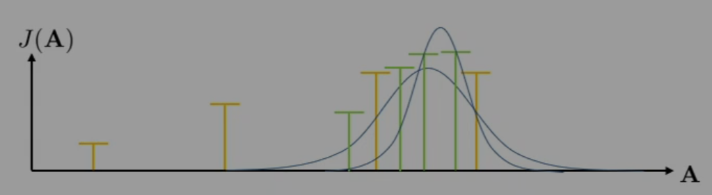
The CEM method is a small modification to stochastic optimization that produces significant performance improvements. In essence, rather than simply sampling $\mathbf{A}_{1},\dots,\mathbf{A}_{N}$ all from some distribution, we sample a set $\mathbf{A}_{1},\dots,\mathbf{A}_{N}$ multiple times. Between iterations, we change our sampling distribution to place more probability mass on the existing "good" samples seen in past iterations. This idea is illustrated below, where the yellow samples are the first iteration, the green samples are the second iteration of samples, and the blue curves represent the changing sample distributions (uniform $\to$ wide curve $\to$ narrow curve).

Here's the algorithm steps.

1. Sample $\mathbf{A}_{1},\dots,\mathbf{A}_{N}\sim p(\mathbf{A})$.
2. Evaluate $J(\mathbf{A}_{1}),\dots,J(\mathbf{A}_{N})$.
3. Pick high-value elites $\mathbf{A}_{i_{1}},\dots,\mathbf{A}_{i_{M}}$ where $M<N$.
4. Refit $p(\mathbf{A})$ to elites $\mathbf{A}_{i_{1}},\dots,\mathbf{A}_{i_{M}}$.

This performs much better than stochastic optimization, while being almost just as simple and still very efficient. Unfortunately, it does still suffer from the curse of dimensionality.

Other Methods

• Monte Carlo tree search (MCTS)
• Continuous trajectory optimization (LQR, etc.)
• Tree-based motion planning (RRT)

How to Plan with Uncertainty

With a deterministic setting, we simply have

In the stochastic setting,

where we are averaging over $N$ samples.

Given the uncertainty of the model, we may use a bootstrap ensemble (see Lecture 15) for $f_{i}$ to reduce distributional shift, which is typically some distribution over deterministic models. Notably, there are two choices for our bootstrap ensemble of when we "sample" a model from the distribution:

1. Sample a single model $f_{i}$ for each $i$, and use it over the whole trajectory
2. Sample a new model $f_{i}$ for every $(i,t)$ (each time step in each trajectory).

However, it typically is more sensible to keep a model constant across a trajectory $(1)$. Otherwise, we're effectively changing our simulated environment every single step—this is bad, because while each environment model in the ensemble is somewhat probable, though perhaps uncertain, a combination of the models, each used at different time steps, may be a very unlikely representation of the environment!

In general, for a candidate action sequence $\mathbf{A}$,

1. Sample $\theta \sim p(\theta \mid \mathcal{D})$ (sample environment model parameters from bootstrap ensemble).
2. At each time step $t$, sample $\mathbf{s}_{t+1}\sim p(\mathbf{s}_{t+1}\mid \mathbf{s}_{t},\mathbf{a}_{t},\theta)$ (sample from environment model).
3. Calculate $R=\sum_{t}r(\mathbf{s}_{t},\mathbf{a}_{t})$.
4. Repeat and accumulate average reward.

This, consequently, computes the value of $J(\mathbf{A})$ for some candidate $\mathbf{A}$ while considering both our epistemic uncertainty about the model's accuracy and the aleatoric uncertainty of the model with regards to the state transitions.

Policy Learning with Models

Let's now return to the stochastic, closed-loop case, or standard RL augmented with an environment model.

Model-free Optimization with a Model

First, we'll discuss how we may simply augment our existing, model-free methods with the use of a model. The simplest approach is to just use policy gradient, but use our model to generate samples.

1. Gather samples from environment model
2. Optimize policy gradient for a few steps
3. Run policy in the real world to generate data to improve our environment model

Notably, though, policy gradient was previously inspired by a lack of knowledge of environment dynamics, and thus relied on samples to estimate $\nabla_{\theta}J(\theta)$—this is known as a likelihood gradient. But, one might notice that, with our environment model's estimate of the dynamics, we can actually perform backpropagation through (the trajectory in) our model to estimate $\nabla_{\theta}J(\theta)$—this is known as a pathwise gradient. Is this better?

The pathwise gradient does reduce variance compared to the likelihood gradient since it is no longer Monte Carlo; however, the pathwise gradient also suffers from severe ill-conditioning due to the multiplication of many (about $H$, the horizon length) Jacobians! Thus, in practice, the standard policy gradient is often more stable than the pathwise gradient, provided sufficient samples.

Key Idea: Backpropagation through learned dynamics generally doesn't perform well due to ill-conditioning.

So, here's our new policy gradient model-based RL algorithm.

1. Run base policy $\pi_{0}(\mathbf{a}_{t}\mid \mathbf{s}_{t})$ to collect $\mathcal{D}=\{ (\mathbf{s},\mathbf{a},\mathbf{s}')_{i} \}$.
2. Learn dynamics model $f(\mathbf{s},\mathbf{a})$ to minimize $\sum_{i}\lVert f(\mathbf{s}_{i},\mathbf{a}_{i})-\mathbf{s}_{i}' \rVert^{2}$.
3. Use $f(\mathbf{s},\mathbf{a})$ to generate trajectories $\{ \tau_{i} \}$ with policy $\pi_{\theta}(\mathbf{a}\mid \mathbf{s})$.
4. Use $\{ \tau_{i} \}$ to improve $\pi_{\theta}$ via policy gradient.
5. $\pi_{0}\leftarrow \pi_{\theta}$.

Note that steps 3-4 are often repeated several times before collecting more data from the real world, to improve sample efficiency.

This method still has some problems, though. In particular, it suffers from the curse of model-based rollouts. In essence, the error caused by distributional shift accumulates quadratically in the length of the horizon. Thus, if we sample long trajectories produced by policy $\pi_{\theta}$ from our dynamics model $f$, the trajectories may become extremely inaccurate!

Thus, we'd like to use our model only for short rollouts. How? We could try simply shortening the task horizon, but for tasks where certain states may only appear in later time steps, this may result in the model never fully learning what it needs. (E.g. model performing a task that is physically impossible to complete within the horizon).

Instead, a more effective method is to generate long rollouts from the real world environment, and then generate short rollouts from $f$ by starting, not from the initial state, but from randomly selected states observed from the real world trajectories (our replay buffer). This reduces our distributional shift error while also allowing the model to see all time steps. However, our state distribution isn't right anymore—our state distribution is now sampled from the states in the replay buffer, which are sampled from older policies. Luckily, our state distribution generally does not diverge too much, and thus this is an acceptable compromise (primarily for off-policy methods, which are more tolerant of this divergence).

So now, here's the modified algorithm.

1. Run base policy $\pi_{0}(\mathbf{a}_{t}\mid \mathbf{s}_{t})$ to collect $\mathcal{D}=\{ (\mathbf{s},\mathbf{a},\mathbf{s}')_{i} \}$.
2. Learn dynamics model $f(\mathbf{s},\mathbf{a})$ to minimize $\sum_{i}\lVert f(\mathbf{s}_{i},\mathbf{a}_{i})-\mathbf{s}_{i}' \rVert^{2}$.
3. Pick states $\mathbf{s}_{i}$ from $\mathcal{D}$, use $f(\mathbf{s},\mathbf{a})$ to generate short rollouts with policy $\pi_{\theta}$.
4. Use both real and model data to improve $\pi_{\theta}$ via off-policy RL.
5. $\pi_{0}\leftarrow \pi_{\theta}$.

This algorithm is very similar to Dyna, which was an early algorithm that performed model-free RL with a model. It's essentially online $Q$-learning augmented with a model.

1. Given state $s$, pick action $a$ using exploratory policy

2. Observe $s',r$ to produce transition $(s,a,s,r')$.

3. Update model $\hat{p}(s'\mid s,a)$ and $\hat{r}(s,a)$ using $(s,a,s')$.

4. Perform $Q$-update (usual Q-learning update)

5. Repeat $K$ times:

   1. Sample $(s,a)\sim \mathcal{B}$, buffer of past states and actions
   2. Perform $Q$-update

This inspired the general "Dyna-style" class of methods.

1. Collect transition data of $(s,a,s,r')$.

2. Learn model $\hat{p}(s'\mid s,a)$, possibly $\hat{r}(s,a)$ too.

3. Repeat $K$ times:

   1. Sample $s\sim \mathcal{B}$, the buffer
   2. Choose action $a$ (from $\mathcal{B},\pi$, or at random)
   3. Simulate $s'\sim p(s'\mid s,a)$, $r=\hat{r}(s,a)$ too if relevant.
   4. Train on $(s,a,s,r')$ with model-free RL.
   5. (Optional) take $N$ more model-based steps to produce short rollout

Note how our algorithm falls into this Dyna-style class.

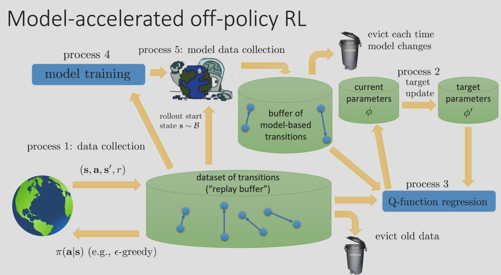
We can generalize these algorithms further as model-accelerated off-policy RL. We can interpret our methods as a composition of several independent processes, similar to $Q$-learning (see [[Lecture 8#More Efficient $Q$-Learning|Lecture 8]]). Note also that we may tune the relative speeds of these processes to produce algorithms with different levels of sample efficiency, learning speed, etc.

1. Data collection from real world
2. Target update
3. $Q$-function regression
4. Dynamics model training
5. Data collection from model

Some actual algorithms that follow this framework:

• Model-Based Acceleration (MBA, Gu et al.)
• Model-Based Value Expansion (MVE, Feinberg et al.)
• Model-Based Policy Optimization (MBPO, Janner et al.)

  Representing the Model

Now, let's discuss the architecture of the dynamics model itself.

Latent State Space Models

Let's consider a partially observed MDP. There is, naturally, some latent state space underlying this MDP. Oftentimes, we'd like to learn this underlying state space, primarily because it may be low-dimensional (relative to the observation space) or it may otherwise simply be easier to run RL on. In particular, we'll be using VAEs (see Lecture 12), which, if you'll recall, attempt to model a latent space $p(\mathbf{z})$ underlying a distribution $p(\mathbf{x})$.

In our case, $\mathbf{x}=(\mathbf{o}_{1},\dots,\mathbf{o}_{H})$ and $\mathbf{z}=(\mathbf{s}_{1},\dots,\mathbf{s}_{H})$. In order to use a VAE, we need to determine our prior $p(\mathbf{z})$. Well, we know that the true distribution $p(\mathbf{z})$ is defined as

We can choose $p(\mathbf{s}_{1})$ to be any (typically simple) distribution, e.g. $\mathcal{N}(0,I)$. However, the probabilities $p(\mathbf{s}_{t+1}\mid \mathbf{s}_{t},\mathbf{a}_{t})$ are the transition probabilities, and thus must be learned—this is the job of our dynamics model.

We also need to determine our decoder $p_{\theta}(\mathbf{x}\mid \mathbf{z})$. Well, based on the structure of the POMDP,

as the observation at time step $t$ is independent of all other states besides the state at time step $t$ (due to the Markovian nature of the states). The separation of the different time steps usually means our decoder is some neural network.

Finally, we need to determine our encoder $q_{\phi}(\mathbf{z}\mid \mathbf{x})$. There are actually many different choices, but one choice is to factor the encoder over time steps (known as a filtering posterior):

Since the encoder takes in all previous observations and actions, and outputs a distribution over states, it's usually some sequence model, e.g. a transformer.

Let's now put these together. We have the following models, which represent our POMDP.

• $p(\mathbf{o}_{t}\mid \mathbf{s}_{t})$: observation model (decoder)
• $p(\mathbf{s}_{t+1}\mid \mathbf{s}_{t},\mathbf{a}_{t})$: dynamics model
• $p(r_{t}\mid \mathbf{s}_{t},\mathbf{a}_{t})$: reward model

And we train our latent space model with

which is just produced by substituting into our previous VAE equations. Note that the expectation is performed w.r.t. $(\mathbf{s}_{t},\mathbf{s}_{t+1})\sim q_{\psi}$.

Choice of Encoder

There's some interesting analysis to be done, though, with regards to our choice of encoder. Recall that we previously chose a filtering posterior

which is a good, simple posterior, but has a major limitation: it treats the distributions of $\mathbf{s}_{t}$ and $\mathbf{s}_{t+1}$ as independent, and since the expectation is taken w.r.t. $(\mathbf{s}_{t},\mathbf{s}_{t+1})\sim q_{\psi}$, we are essentially computing the expectation with respect to all pairs of states $(\mathbf{s}_{t},\mathbf{s}_{t+1})$ sampled from our model! In reality, though, each $\mathbf{s}_{t}$ is only likely to transition to a much smaller subset of possible $\mathbf{s}_{t+1}$'s.

This gives rise to a common problem in variational inference known as posterior collapse, in which insufficient dependencies between the latent variables induces erroneously $q_{\psi}(\mathbf{z}\mid \mathbf{x})\approx p(\mathbf{z})$. The idea is that the filtering posterior has difficulty learning because it's attempting to learn a transition between two independent states; therefore, the encoder simply decides to minimize the divergence penalty rather than the "reconstruction" penalty, since it cannot effectively minimize the reconstruction penalty.

While this can be problematic, in instances where the observations already capture much of the state, and what's really desired is the use of VAE to disentangle the underlying factors of variation of the state and learn a nicer representation of the state, this works fine!

However, if this is a limitation for the problem, there are other posteriors we can use. In particular, the full smoothing posterior

which takes as input the actions and observations over the entire horizon. This is, of course, a more complex model. However, now the dynamics model will receive samples $(\mathbf{s}_{t},\mathbf{s}_{t+1})\sim q_{\psi}$ that are highly correlated, and can more easily learn.

Alternatively, we can go to the opposite extreme, if we desire an even simpler model, and use a single-step encoder:

This is okay if we are in an almost fully observed MDP, i.e. each observation almost entirely capture its corresponding state.

Generally speaking, the filtering posterior is the most balanced choice, but the choice of encoder can change depending on the problem. (The single-step encoder and filtering posterior are pretty common).

Simple Latent Space Model Analysis

What if we wanted to make the simplest latent space model? We'll use a single-step encoder, and we will even define $q_{\psi}(\mathbf{s}_{t}\mid \mathbf{o}_{t})$ to be deterministic. In other words,

for some function $g_{\psi}$. (Note that $\delta$ is the Dirac delta function, and represents the concentration of all probability mass at a single point).

Now, let's analyze our training equation. First, we can remove our expectation and substitute in $g_{\psi}$ everywhere $\mathbf{s}$ was used, since $q_{\psi}$ is now deterministic. Additionally, we may delete the entropy term from the expression since it is effectively useless now; $g$ is a Dirac delta function and thus its entropy (which is technically $-\infty$, FYI) cannot change.

Intuitively, this is saying that, w.r.t $\psi$ and $\phi$, we maximize the probability of $g_{\psi}(\mathbf{o}_{t,i})$ decoding back to $\mathbf{o}_{t,i}$ (second term) and the probability that $g_{\psi}$ obeys the learned dynamics (first term), over all trajectories and time steps. This should make sense!

Of course, without any uncertainty or handling of partial observability, this only really works when you just desire a compact representation/encoding of your state.

Actor-Critic with Learned Representations

We can add these latent state space models to our existing model-free methods, like actor-critic, to produce an actual algorithm.

1. Get $(\mathbf{o}_{i},\mathbf{a}_{i},\mathbf{o}_{i}')$ by taking one step with $\mathbf{a}\sim \pi_{\theta}(\mathbf{a}\mid \mathbf{o})$, store in replay buffer $\mathcal{R}$.
2. Update the model: $p_{\phi}(\mathbf{s}_{t+1}\mid \mathbf{s}_{t},\mathbf{a}_{t})$, $p_{\phi}(r_{t}\mid \mathbf{s}_{t})$, $p(\mathbf{o}_{t}\mid \mathbf{s}_{t})$, $q_{\psi}(\mathbf{s}_{t}\mid \mathbf{o}_{t})$ using a batch $\sim \mathcal{R}$.
   (dynamics, reward, decoder, and encoder models, respectively)
3. Infer $\mathbf{s}_{i}\sim q_{\psi}(\mathbf{s}_{i}\mid \mathbf{o}_{i})$ and $\mathbf{s}_{i}'\sim q_{\psi}(\mathbf{s}_{i}',\mathbf{o}_{i}')$. (Note that $\mathbf{s}_{i},\mathbf{s}_{i}'$ may be encoded jointly if using a full smoothing posterior).
4. Evaluate target value $y_{i}=r(\mathbf{s}_{i},\mathbf{a}_{i})+\gamma \mathbb{E}_{\mathbf{a}'\sim \pi_{\theta}(\mathbf{a}'\mid \mathbf{o}_{i}')}[\hat{Q}_{\phi}^{\pi}(\mathbf{s}_{i}',\mathbf{a}')]$.
5. Approximate $\nabla_{\theta}J(\theta)$ with e.g. reparameterized policy gradient.
6. $\theta\leftarrow\theta+\alpha \nabla_{\theta}J(\theta)$.

Actor-Critic with Model-Based RL

Returning to the ideas in [[#Policy Learning with Models]], we can produce an actor-critic algorithm that uses the dynamics model to simulate more data.

1. Get $(\mathbf{o}_{i},\mathbf{a}_{i},\mathbf{o}_{i}')$ by taking one step with $\mathbf{a}\sim \pi_{\theta}(\mathbf{a}\mid \mathbf{o})$, store in replay buffer $\mathcal{R}$.

2. Update the model: $p_{\phi}(\mathbf{s}_{t+1}\mid \mathbf{s}_{t},\mathbf{a}_{t})$, $p_{\phi}(r_{t}\mid \mathbf{s}_{t})$, $p(\mathbf{o}_{t}\mid \mathbf{s}_{t})$, $q_{\psi}(\mathbf{s}_{t}\mid \mathbf{o}_{t})$ using a batch $\sim \mathcal{R}$.
   (dynamics, reward, decoder, and encoder models, respectively)

3. Infer $\mathbf{s}_{i}\sim q_{\psi}(\mathbf{s}_{i}\mid \mathbf{o}_{i})$ and $\mathbf{s}_{i}'\sim q_{\psi}(\mathbf{s}_{i}',\mathbf{o}_{i}')$. (Note that $\mathbf{s}_{i},\mathbf{s}_{i}'$ may be encoded jointly if using a full smoothing posterior).

   1. Simulate additional data with $p_{\phi}$.
   2. Evaluate target value $y_{i}=r(\mathbf{s}_{i},\mathbf{a}_{i})+\gamma \mathbb{E}_{\mathbf{a}'\sim \pi_{\theta}(\mathbf{a}'\mid \mathbf{o}_{i}')}[\hat{Q}_{\phi}^{\pi}(\mathbf{s}_{i}',\mathbf{a}')]$.
   3. Update $\phi$ with $\nabla_{\phi}\sum_{i=1}^{B}\lVert \hat{Q}_{\phi}^{\pi}(\mathbf{s}_{i},\mathbf{a}_{i})-y_{i} \rVert^{2}$.
   4. Approximate $\nabla_{\theta}J(\theta)$ with e.g. reparameterized policy gradient.
   5. $\theta\leftarrow\theta+\alpha \nabla_{\theta}J(\theta)$.