Lecture 17: Offline Reinforcement Learning

Introduction

Recall on-policy and off-policy RL. In both classes of algorithms, data is collected by running a policy in the real-world/simulator (off-policy RL collects more data to add to the replay buffer). Offline RL is somewhat similar to off-policy RL, except the replay buffer is static; no additional data is collected during training.

First off, how is this even possible? RL is seemingly centered around this "trial and error" approach that allows a model to test policies in the real-world and subsequently optimize. Intuitively, it's because

Offline RL finds the "good behaviors" in a static dataset
Good behavior in one region may suggest good behavior in another region
Components of good behavior can be "stitched" together to produce more complex, good behavior

Notably, offline RL also differs from imitation learning in that the dataset may not consist of optimal trajectories! Offline RL makes no assumption about the quality of the dataset.

Distributional Shift

First, we will assume our dataset $\mathcal{D}$ is generated by some policy $\pi_{\beta}$ , and that we are maximizing the usual, discounted RL objective w.r.t. policy $\pi_{\theta}$

\max _{\theta}\sum_{t=0}^{H} \mathbb{E}_{\mathbf{s}_{t},\mathbf{a}_{t}\sim \pi_{\theta}(\mathbf{a}\mid \mathbf{s})}[\gamma^{t}r(\mathbf{s}_{t},\mathbf{a}_{t})]

Unfortunately, running any of our usual model-based or model-free RL algorithms will run into serious distributional shift problems between our behavior policy and our target policy. This is actually a "surface symptom" of a deeper, more fundamental problem: counterfactual queries. Counterfactual questions ask about "what if" scenarios; in RL, this means determining how good some action is when it's never been seen before in training data. With online RL, this is resolved by simply trying out the action; in offline RL, this is not possible. So, how do effectively generalize in offline RL to unseen data?

Intuitively, distributional shift occurs because RL methods inherently maximize when producing some policy evaluation or policy prediction function; this encourages maximization even over the errors of the model, like what we saw in [[Lecture 8#Overestimation in $Q$ -Learning|Lecture 8]] with $Q$ -learning. (If minimizing a function, e.g. loss, still maximizing error; just in the other direction). Moreover, techniques like importance sampling in off-policy RL methods that correct for the divergence between distributions typically incur high variance (for importance sampling, this is due to the multiplication of many importance ratios).

However, off-policy RL methods like PPO typically include some term in the objective function that constrains distribution divergence, i.e. a KL divergence term. This is known as a policy constraint, and, as we'll soon see, some type of policy constraint exists in practically all offline RL methods.

In short, the existing challenges with sampling error and function approximation in standard RL become more severe in offline RL.

Policy Constraints

First, there a few principles for offline RL that, empirically, have proved effective.

Use value-based/model-based methods.
Somehow fix distributional shift
- Policy constraints
- Pessimism
- Avoid out-of-distribution actions in updates

A simple policy-constrained offline RL algorithm can be derived just from a standard off-policy policy gradient.

J(\theta)=\mathbb{E}_{\mathbf{a}\sim \pi_{\theta}(\mathbf{a}_{t}\mid \mathbf{s}_{t}^{(i)})}[Q^{\pi}(\mathbf{s}_{t}^{(i)},\mathbf{a}_{t})]+\alpha D_{\text{KL}}(\pi_{\beta}(\mathbf{a}_{t}\mid \mathbf{s}_{t}^{(i)})\parallel \pi_{\theta}(\mathbf{a}_{t}\mid \mathbf{s}_{t}^{(i)}))

Actually, we can also use the reverse KL divergence, which swaps $\pi_{\beta}$ and $\pi_{\theta}$ , instead of the forward KL divergence. Is there a difference? Well, the two are, mathematically,

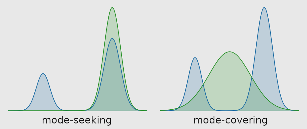
\begin{align*} D_{\text{KL}}(\pi_{\beta}\parallel \pi_{\theta}) &= -\mathbb{E}_{\mathbf{a}\sim \pi_{\beta}(\mathbf{a}\mid \mathbf{s})}[\log \pi_{\theta}(\mathbf{a}\mid \mathbf{s})] - \mathcal{H}(\pi_{\beta}(\mathbf{a}\mid \mathbf{s})) \\ D_{\text{KL}}(\pi_{\theta}\parallel \pi_{\beta}) &= -\mathbb{E}_{\mathbf{a}\sim \pi_{\theta}(\mathbf{a}\mid \mathbf{s})}[\log \pi_{\beta}(\mathbf{a}\mid \mathbf{s})] - \mathcal{H}(\pi_{\theta}(\mathbf{a}\mid \mathbf{s})) \end{align*}

Consider the first equation, i.e. forward KL divergence. First, note that the entropy term is essentially just an additive constant, since changing $\theta$ does not change the entropy of the distribution $\pi_{\beta}$ . For any sample that has a probability of $0$ under $\pi_{\theta}$ and a nonzero probability under $\pi_{\beta}$ , the overall expression diverges to $-\infty$ ; in other words, an extremely harsh penalty for assigning a probability of $0$ to any sample in $\pi_{\beta}$ . Meanwhile, it doesn't significantly encourage the assignment of higher probabilities to any samples; thus, this induces the assignment of moderate probabilities to most actions. This leads to a phenomenon known as mode covering, in which $\pi_{\theta}$ generates a broader distribution to cover all the data.

In contrast, reverse KL divergence encourages $\pi_{\theta}$ to choose actions that are high probability in $\pi_{\beta}$ , and doesn't strongly penalize for perhaps missing out on other actions. And, for any sample that has a probability of $0$ under $\pi_{\beta}$ , the overall expression diverges to $-\infty$ ; in other words, an extremely harsh penalty for assigning a nonzero probability to any sample with $0$ probability under $\pi_{\beta}$ . This encourages mode seeking, in which $\pi_{\theta}$ generates a narrower distribution to cover a specific, high-probability mode of the distribution.. An illustration of mode seeking vs. mode covering is shown below.

Why choose one over the other?

Forward KL
- Avoids reward hacking
- Good if we don't know $\pi_{\beta}$ (reuse samples)
- Good if we don't want to lose some modes (e.g. LLM)
Reverse KL
- Avoids unobserved actions
- Good if you want the "best mode inside data"
- Good with max-entropy RL
- Requires estimating $\pi_{\beta}$

Typically, though, forward KL is chosen because it's simply much easier to implement!

As a sidenote, one may use non-KL-based policy constraints, e.g.

D_{\text{support}}(\pi_{\theta}(\mathbf{a}\mid \mathbf{s}),\pi_{\beta}(\mathbf{a}\mid \mathbf{s}))=\mathbb{E}_{\mathbf{a}\sim \pi_{\theta}(\mathbf{a}\mid \mathbf{s})}[\delta(\pi_{\beta}(\mathbf{a}\mid \mathbf{s})=0)]

which essentially allows assigning probability in $\pi_{\theta}$ to only states seen in $\pi_{\beta}$ , and has no additional term to encourage entropy in the distribution. Due to practical challenges (difficult to approximate tractably), though, such a constraint has seen limited use.