for the forward and reverse KL divergence, respectively. Generally, this is not the best way to add policy constraints, but it can work well if done right.
We can also instead modify the reward function. Typically, this is done with reverse KL + MaxEnt RL.
r^(s,a)=r(s,a)−λDKL=r(s,a)+λlogπβ(a∣s)
This is particularly interesting because it also accounts for future divergence.
Now, we can construct some real offline actor-critic algorithms.
Here's a BRAC-like, behavior regularized actor critic, algorithm. (Behavior Regularized Offline Reinforcement Learning, Wu et al.)
J(θ)=∑iEa∼πθ(a∣s,i)[Q^ϕπ(si,a)]+λlogπθ(ai∣si). (modifying actor objective with forward KL)
θ←θ+α∇θJ(θ).
Implicit Policy Constraint Methods
info
From papers like Advantage-Weighted Regression (Peng et al.) and Accelerating Online Reinforcement Learning with Offline Datasets (Nair et al.). (Both advised by Levine orz).
Implicit policy constraint methods do not add an explicit regularizer term.
Consider, for instance, finding the optimal policy πnew over expectation of a Q-function, subject to a reverse KL divergence constraint.
π∗=πargmaxEa∼π(a∣s)[Q(s,a)],DKL(π∥πβ)≤ϵ
Via classical convex optimization techniques, we can derive an exact, closed-form answer. (Note: this is usually not practical due to the size of the action space).
π∗(a∣s)=Z(s)1πβ(a∣s)exp(λ1Aπ(s,a))
Now, the idea is that we can use importance sampling to effectively approximate samples from π∗ using samples from πβ, and then use behavioral cloning (supervised learning) to learn from the samples of π∗. In particular, we approximate via importance-weighted maximum likelihood, i.e. we produce an update rule
where all terms not dependent on θ were removed, is equivalent to learning a policy πθ that behaviorally clones the optimal policy π∗ under the reverse KL divergence constraint.
This may translate to an AWAC-like, advantage-weighted actor-critic, algorithm. (Nair et al.)
Note that you can also approximate V^π(si)≈Qϕπ(si,a) where a∼πθ(a∣si) if you don't want to train a separate neural network to learn V^π.
This approach is nice for its simplicity; however, it is limited primarily by the fact that, in copying the samples generated by the behavioral policy, it is slow to learn to avoid bad actions.
Implicit Q-Learning (IQL)
info
Paper: Offline Reinforcement Learning with Implicit Q-Learning (Kostrikov et al.). (Also Levine).
Here's a thought: what if we simply avoided all out-of-distribution actions when performing our Q-update? (Q-update needs to maximize over all actions). The intuition is that neural networks can often generalize very well to unseen actions, without explicit consideration of such actions.
Consider performing policy evaluation of the behavior policy. With a typical MSE loss, we might have
which simply regresses onto the mean of the value of each state/action under the behavior policy. However, we can actually regress onto an upper quantile of these values instead, by changing our loss function.
V=Vmin(s,a)∈D∑ℓτ(V(s)−Q(s,a))
where ℓτ is a function that heavily penalizes V underestimating Q, and softly penalizes V overestimating Q. It's essentially just MSE with a multiplier on all negative values in the domain. This essentially induces our function estimator to perform implicit maximization over the actions in estimating the value function.
Doesn't this cause erroneous overestimation? Wasn't this an issue in soft actor-critic?
Actually, no. In SAC, overestimation was caused by optimism towards the state transitions. Here, the Q-function estimator still uses standard MSE to effectively regress onto the state transitions. Only the V estimator now uses the modified loss function to implicitly maximize over the actions—which is precisely what we want for an RL algorithm. It would overestimate had we implemented, say, implicit maximization with just a Q-function. (That is, the Q-function's use of standard MSE ensures no erroneous overestimation).
Note that it is actually possible to show that this is essentially equivalent to Q-learning with Q-updates that maximize only over actions seen in the sample data of the behavioral policy.
Thus, here's an offline-actor critic algorithm with implicit Q-learning.
Evaluate yi=r(si,ai)+γV^ψ(si).
Update ϕ using ∇ϕ∑i=1B∥Q^ϕ(si,ai)−yi∥2.
Update ψ using ∇ψ∑i=1Bℓ2τ(V^ψ(si)−Q^ϕ(si,ai)).
J(θ)=∑ilogπθexp(Q^ϕ(si,ai)−V^ψ(si)).
θ←θ+α∇θJ(θ).
Some interesting things to note:
No expectations under πθ.
Actor and critic are completely independent.
Conservative Q-Learning (CQL)
info
Paper: Conservative Q-Learning for Offline Reinforcement Learning (Kumar et al.). (Yes, also Levine).
Let's now return to the idea of pessimism to solve distributional shift.
Our inspiration is to apply some ideas from adversarial training. Let's redefine our Q function as
where the first term "pushes down" on large Q-values, and the second term is just our regular Q-learning objective. (μ is our discriminator, the policy π is our generator, in GAN terms). Note that one may show that Q^π≤Qπ for large enough α, or that our Q^π is a lower bound on the actual Q function.
There's one issue with this solution, though—this will produce a systematic underestimate on actions close to the data. A better estimate is
This new term essentially just pushes back up on (s,a) samples in our data, and effectively cancels out with the first term. Notably, we no longer have the guarantee that Q^π≤Qπ for all(s,a), but we are guaranteed that Eπ(a∣s)[Q^π(s,a)]≤Eπ(a∣s)[Qπ(s,a)] for all s∈D.
Thus, we have a basic conservative Q-learning algorithm.
Update Q^π w.r.t. LCQL(Q^π) using D.
Update policy π, dependent on discrete/continuous action space.
We've left something out though in our discussion so far—what is this μ term? Well, it's the distribution that maximizes that inner term; however, without any regularization, it's extremely unstable over the course of training. Typically, we'll add a regularization term R(μ) to the loss function, i.e.
A common choice for R(μ) is Es∼D[H(μ(⋅∣s))], or maximum entropy regularization. In this case, after learning, μ becomes proportional to exp(Q(s,a)). Notably, we can either represent μ as an actual, explicit learned policy, or we can note that
Ea∼μ(a∣s)[Q(s,a)]=loga∑exp(Q(s,a))
For discrete actions, we can calculate this quantity directly, while for continuous actions, we can use importance sampling to estimate this quantity.
What if you didn't use a regularizer?
If you didn't add a regularizer R(μ), the maximizing μ is a distribution that assigns probability 1 to the highest Q-value. Because this may change between every iteration, it is potentially unstable, and therefore slows learning. With maximum entropy regularization, the distribution is encouraged to spread out a bit more over the large Q-values.
Offline-to-online RL
Now, let's turn to the problem of offline-to-online RL: using offline RL to pretrain a model, and then using online RL to fine-tune the model.
At the time of writing (March 2026), this is an active area of research. Take all following discussions with a grain of salt.
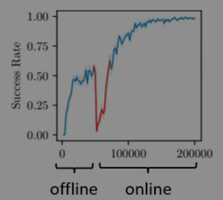
Okay, so what if we just run an offline RL algorithm, e.g. CQL, and then run a standard online RL algorithm starting from the same point (same policy, same Q-function)? Does that just work?
Unfortunately, not quite. See below.
For CQL, in particular, which this graph was generated from, during the first phase of online training, the model will realize that it has drastically underestimated the Q-function for some previously unobserved actions, due to the pessimism of CQL. Other offline RL algorithms have similar, slightly different versions of this same problem.
The problem is the differences between the training phases.
Offline:
Stay close to πβ.
Conservative values (e.g. Q^π≤Qπ).
Lots of gradient steps on the same data.
Online:
Improve as much as possible over πβ.
Optimistic values (e.g. Q^π≥Qπ). (important for exploration)
Learn as quickly as possible.
There is, notably, an "embarrassingly effective" method that is not really offline RL at all, yet outperformed, for a long time, many offline RL methods in using offline data for online methods. (Efficient Online Reinforcement Learning with Offline Data, Ball et al.).
Initialize two buffers: online replay buffer and offline data buffer
Initialize value function and actor from scratch.
Run online RL; for every batch, sample half from offline buffer and half from replay buffer.
Obviously, this method is unsatisfying because it involves absolutely zero pretraining. Unfortunately, there isn't a clear solution to this; however, in recent years, algorithms that use diffusion models or flow matching to represent the actor have empirically produced methods with pretraining that do improve over the "embarrassingly effective" method.
It's unknown why exactly they work well, but here is one theory. In the online case, optimal πθ(a∣s) is deterministic; thus, there's no need to capture some multimodal distribution for the policy. In the offline case, capturing only the best mode in the data is fine... but when capturing multiple modes, it may be easier to handle policy constraints. So, for offline-to-online, perhaps it helps to just track all the modes in the offline phase, and then focus on the best mode in the online phase.
However, it's hard to use diffusion as the actor in RL. Optimizing the objective requires either ∇θlogπθ(a∣s) (policy gradient) or backpropagation through the diffusion process (reparameterization). Policy gradient is inaccessible for diffusion/flow matching, and backprop is often computationally expensive and unstable (backprop through time, BPTT).
Let's discuss some methods that have used diffusion models, and what they did to solve the above issue.
IDQL
Simple offline-to-online RL with diffusion model. (IDQL: Implicit Q-Learning as an actor-critic method with diffusion policies, Hansen-Estruch et al.)
Train Q^ϕ(s,a) without any actor (e.g. IQL)
Train πθ(a∣s) as a diffusion/flow model with behavioral cloning, leads to πθ≈πβ.
At test time, sample {a1,…,aK} from πθ(a∣s), and pick argmaxakQ^ϕ(s,ak).
The point is that no out-of-distribution actions are chosen because πθ≈πβ. This is somewhat reminiscent of stochastic optimization/random shooting from Lecture 16. However, this works surprisingly well, particularly if the data produced by πβ is somewhat decent.
FQL
An actor that stays "close" to diffusion model. (Flow Q-Learning, Park et al.)
Train πflow(a∣s,z) as diffusion/flow model with behavioral cloning, where z is the input noise in flow matching. This leads to πflow≈πβ.
Run offline actor-critic with a special behavioral cloning regularizer, training the actor πθ(a∣s,z) to stay close to πflow(a∣s,z), given both s and z as input. Notably, the actor is just a regular neural network, not a flow model, that is essentially distilling the behavior of the flow model. In particular, the objective for the actor is
Diffusion Steering via Reinforcement Learning. (Steering Your Diffusion Policy with Latent Space Reinforcement Learning, Wagenmaker et al.)
Intuitively, a diffusion model actually produces an action space of only in-distribution actions. So, what if, instead of our actor model producing an action from the general action space, which may be out-of-distribution, we use our actor model to produce a value in the latent space of the diffusion model, i.e. the noise distribution, and then feed that into the diffusion model to produce an in-distribution action. That is, just run an efficient online RL algorithm in the latent space of a diffusion model!
Model-based Offline RL
The critical concern in model-based offline RL is that we'd like to limit the impact of the distributional shift of the environment model itself, because we are unable to collect more data to correct the model's errors. (counterfactual questions for the model, rather than for the Q-function like previously).
MOPO
MOPO: Model-Based Offline Policy Optimization (Yu et al.)
Also, MOReL: Model-Based Offline Reinforcement Learning (Kidambi et al.)
One solution is to simply adjust the reward function to be pessimistic about OOD states, i.e. to "punish" the policy for exploiting OOD states. The reward is adjusted as follows
r~(s,a)=r(s,a)−λu(s,a)
where u(s,a) represents an uncertainty penalty. This can be computed by e.g. measuring disagreement between ensemble models. Subsequently, simply run any existing model-based RL method.
COMBO
COMBO: Conservative Offline Model-Based Policy Optimization (Yu et al.)
Alternatively, we can leverage the same ideas as in [[#Conservative Q-Learning (CQL)|CQL]]. Similar to how CQL "pushes down" on large Q-values, model-based RL can "push down" on the Q-values of model state-action tuples. In essence, for a model p, we use a Q-function update rule of
Again, the intuition is the same. It's like a GAN: if the model, the generator, produces something that looks clearly different from real data, the Q-function, the discriminator, will assign low values to it.