Chapter 10: Sequence Modeling: Recurrent and Recursive Nets

Recurrent neural networks, or RNNs, are networks designed to process sequential data. An RNN may be imagined to be recursing cyclically on a single layer or subcomponent of the greater model; really, it's essentially just an application of parameter sharing to regular feedforward networks!

10.1 Unfolding Computational Graph

As aforementioned, RNNs have a cyclical or recursive structure. In particular,

In other words, the hidden layer for time step $t$ is a function of the previous hidden layer for time step $t-1$ and the $t$th value in the input sequence. For such a network, there are two possible representations as a computational graph, shown below.

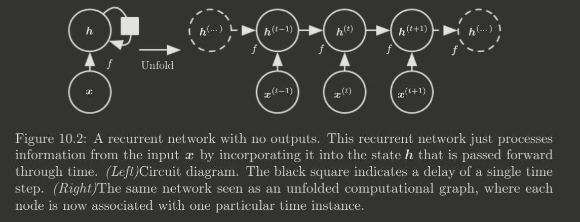
The unfolded representation has the advantage of allowing us to represent the function underlying $\boldsymbol{h}^{(t)}$

as the repeated application of a function $f$. This is important because

• Regardless of sequence length, the learned model has the same input size, since it is defined in terms of $f$ not $g$.
• The transition function $f$ and its parameters may be reused

This enables generalization to arbitrary sequence lengths.

10.2 Recurrent Neural Networks

Below displays the structure of the basic RNN.

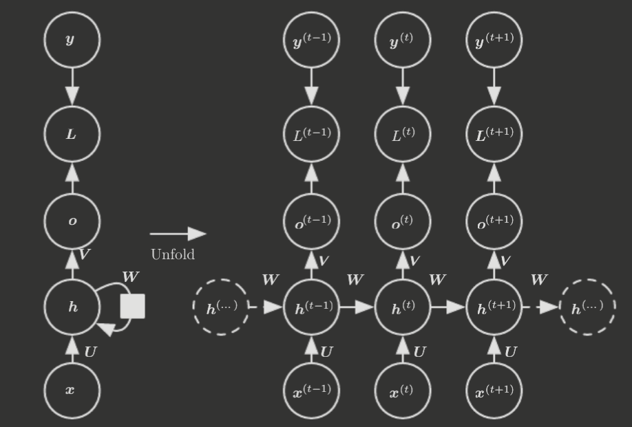
This is what we will typically use to discuss RNNs. Before proceeding, however, we note some other important RNN structures.

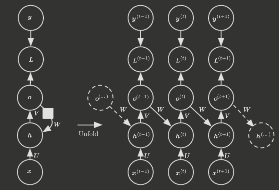
There are RNNs that similarly produce an output at each time step, but have recurrent connections only from $\boldsymbol{o}^{(t-1)}\to \boldsymbol{h}^{(t)}$.

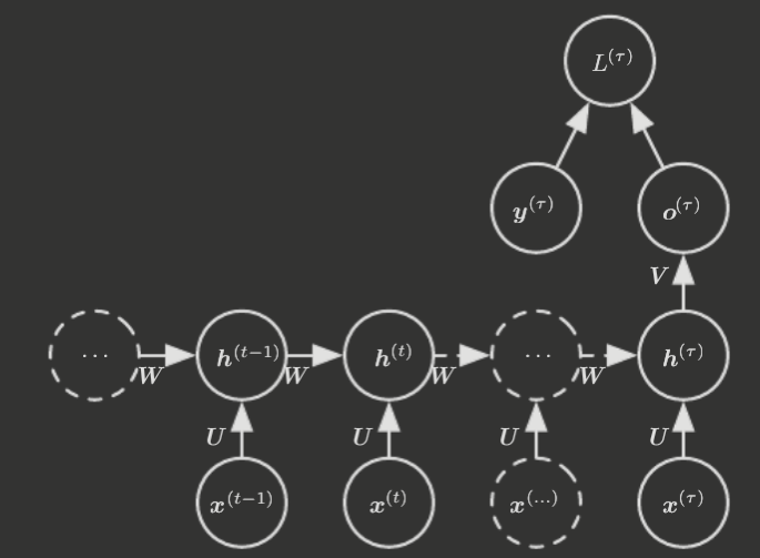
And there are RNNs that only produce one output at the end of the sequence.

Now, returning to the basic RNN structure, let's consider how we would train the network. Given some output sequence $\boldsymbol{y}$ and some input sequence $\boldsymbol{x}^{(1)},\dots,\boldsymbol{x}^{(t)}$, the negative log-likelihood is

Computing the gradient of this expression is very expensive, as it requires back-propagating through all time steps $t$. (In fact, it is known as back-propagation through time (BPTT)). Can we do better?

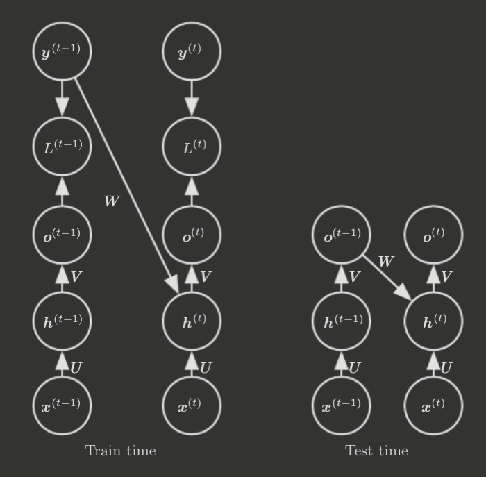
Teacher Forcing and Networks with Output Recurrence

Recall the RNN structure with only recurrent connection from $\boldsymbol{o}^{(t-1)}\to \boldsymbol{h}^{(t)}$. It is a less powerful model because it lacks hidden-to-hidden recurrence, and thus relies on the output units to capture all information about the past, which is generally less effective since the model is trained to match the output to the training set targets.

However, this structure has a key advantage—the time steps are all decoupled for back-propagation! The idea is that the training set already provides the ideal value of $\boldsymbol{o}^{(t-1)}$; therefore, the gradient computation can be parallelized, with each time step being handled independently by using the training set's ideal $\boldsymbol{o}^{(t-1)}$ to train $\boldsymbol{h}^{(t)}$.

This method can be extended to the forward propagation process too, in what is known as teacher forcing. In essence, instead of feeding $\boldsymbol{o}^{(t-1)}$ through the recurrent connection as input for $\boldsymbol{h}^{(t)}$, we use $\boldsymbol{y}^{(t-1)}$.

This is not actually motivated by efficiency goals, however (though it does allow parallel computation of forward propagation too). Instead, it derives directly from maximum likelihood estimation. Consider, for instance, a two-step sequence. The maximum likelihood criterion is

Since $\boldsymbol{y}^{(2)}$ is dependent on $\boldsymbol{y}^{(1)}$, this is equivalent to

In other words, the target values should be used for the next input layer, and thus maximum likelihood estimation implies the use of teacher forcing.

Computing the Gradient in a Recurrent Neural Network

BPTT, in reality, just requires applying backward propagation through the unrolled computational graph.

Recurrent Neural Networks as Directed Graphical Models

Most of this section essentially describes thinking about RNNs in terms of their unrolled computational graphs. There are a couple key ideas, though.

RNNs possess an efficient parameterization of the unrolled graphical model, with their parameter sharing. However, this can cause difficulties in parameter optimization; in particular, it expresses a strong prior over the model that assumes the conditional probability distribution $p(\boldsymbol{v}_{t+1}\mid \boldsymbol{v}_{t})$, where $\boldsymbol{v}_{t}$ represents all variables (hidden units, output units, etc.) at time $t$, is stationary, i.e. it does not depend on $t$.

Also, we must consider how an RNN decides when to stop producing output. There are a number of ways to do this.

• If the output is some vocabulary, a special stop symbol may be used.
• An extra Bernoulli output that decides whether to continue generation or halt generation.
• An extra output that predicts the sequence length itself. Note that this requires an extra input for each recurrence step to give the model context of its position in the sequence. (Otherwise, the sequence may abruptly stop).

Modeling Sequences Conditioned on Context with RNNs

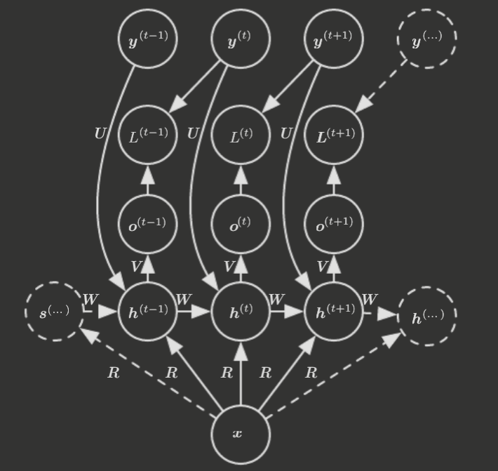
Sometimes, rather than taking a sequence of vectors $\boldsymbol{x}^{(t)}$ as input, the RNN receives a single, fixed-length vector $\boldsymbol{x}$. Then, it's common to do one of a few things.

• Add $\boldsymbol{x}$ as an extra input to every time step.
• Use it as the initial state $\boldsymbol{h}^{(0)}$.
• Both!

The first approach is displayed below.

10.3 Bidirectional RNNs

Thus far, the RNNs we've seen have had a causal structure, in which the state at time $t$ only captures past information and the current input. However, many problems require outputs that depend on the whole input sequence. Bidirectional RNNs enable this by essentially combining a feed-forward RNN (moves forward in time) with a feed-backward RNN (moves backward in time). This allows the state at time $t$ to consider information from both the past and the future.

10.4 Encoder-Decoder Sequence-to-Sequence Architectures

Thus far, we have discussed RNN architectures that

• Map a variable-length sequence to a fixed-size vector
• Map a fixed-size vector to a variable-length sequence
• Map a variable-length sequence to a sequence of the same length

However, what if want to map a variable-length sequence to a sequence of a different, variable length?

The simplest architecture for such a task is the encoder-decoder architecture. In essence, an encoder RNN process the input sequence, and produces a fixed-length context vector $C$ that is effectively a representation of the input for the model. Then, a decoder RNN processes the context $C$ to produce the variable-length output sequence. Note that the context $C$ is commonly the last hidden state of the encoder RNN.

This architecture, however, is flawed in its choice of $C$ to be fixed-length; in some cases, $C$ may be too small to properly represent a long sequence. A paper from Bahdanan et al. addressed this, both modifying $C$ to be variable-length and introducing the now famous attention mechanism.

10.5 Deep Recurrent Networks

RNNs can typically be broken down into three blocks of parameters and associated transformations.

• Input $\to$ Hidden
• Hidden$^{(t)}$ $\to$ Hidden$^{(t+1)}$
• Hidden $\to$ Output

In our basic RNN architecture, each block is just one weight matrix. However, just like with feedforward networks, we need not be limited to one layer—we can introduce depth to produce deep RNNs. This can be done in various ways:

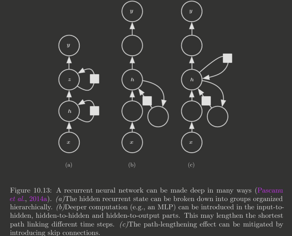
One idea $(a)$ is to have a deep neural network with multiple layers being recurrent with themselves. Another $(b)$ is to have a deeper MLP in each block. Notably, $(b)$ increases the length of the state-to-state transition, and thus optimizations such as skip connections (which skip the deeper layers) may be introduced $(c)$.

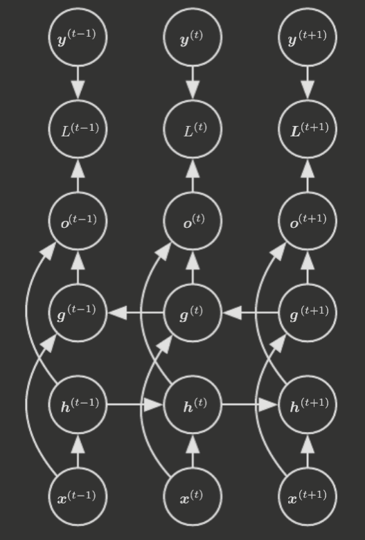
10.6 Recursive Neural Networks

Recursive neural networks are a generalization of recurrent neural networks, in which the computational graph structure is tree-like rather than the chain-like structure of RNNs. For instance, see below.

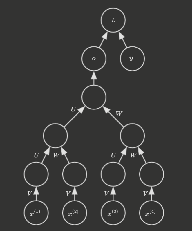
One notable advantage of recursive nets, relative to RNNs, is that for a sequence of length $\tau$, the depth (i.e. distance from any one input to the output) is reduced from $O(\tau)$ to $O(\log \tau)$, which improves long-term dependencies.

It remains, however, an open question (at the time of this book's writing) how best to structure the tree itself, which, ideally, should be learned.

10.7 The Challenge of Long-Term Dependencies

The key issue is that gradients propagated over many stages tend to vanish (or explode, but very rarely). Thus, the model appears to "forget" earlier components of the input sequence. This derives naturally from the structure of RNNs, with parameters being applied exponentially.

Formally, if $\boldsymbol{W}$ is the weight matrix describing the hidden-to-hidden recurrence relation, and it has eigendecomposition $\boldsymbol{W}=\boldsymbol{Q}\boldsymbol{\Lambda}\boldsymbol{Q}^{\top}$, then

Any eigenvalues with $\lvert \lambda \rvert>1$ will explode, while those with $\lvert \lambda \rvert<1$ will vanish as $t_{2}-t_{1}\to \infty$. Eventually, any component of $\boldsymbol{h}^{(t_{2})}$ not aligned with the largest eigenvector will become irrelevant.

10.8 Echo State Networks

Echo state networks (ESNs) (and liquid state machines, the equivalent of ESNs with binary neurons instead of continuous neurons) are a type of recurrent model that attempt to manually set the hidden units to capture historical information well, and only train the output weights. This is known as reservoir computing, as the hidden units essentially form a "reservoir" of temporal features.

One may imagine reservoir RNNs as much like kernel machines—they map a variable-length sequence into a fixed-length sequence, upon which a linear predictor may be applied.

Then, of course, the challenge is to determine the right input and recurrent parameter values. The idea, typically, is to view the RNN as a dynamical system, and set the parameters appropriately to achieve near-stability. In particular, the original idea was to ensure the Jacobian of the state-to-state transitions function have eigenvalues be close to 1; in particular, it was desirable to keep the spectral radius of $\boldsymbol{J}^{(t)}$, $\underset{i}{\max}\ \lvert \lambda_{i} \rvert$, small.

Considering a linear network, i.e. $\boldsymbol{h}^{(t+1)}={\boldsymbol{h}^{(t)}}^{\top}\boldsymbol{W}$, we say that a linear map $\boldsymbol{W}$ is contractive if it shrinks $\lVert \boldsymbol{h} \rVert_{2}$. This occurs if $\boldsymbol{J}^{(t)}<1$, and actually may help the network forget unnecessary information; which is a must considering the finite precision of the state vector.

With a nonlinear network, the Jacobian may change across steps; in fact, a squashing nonlinearity such as $\tanh$ can bound the recurrent dynamics (for exploding $W$ with spectral radius $>1$)!

10.9 Leaky Units and Other Strategies for Multiple Time Scales

One methodology for remembering long-term dependencies is to design a model where separate subcomponents operate at different time scales—some fine-grained, others coarse time scales. There are several techniques to implement this.

Adding Skip Connections through Time

Skip connections directly connect variables from time step $t_{1}$ to variables in time step $t_{2}$, where $t_{2}-t_{1}$ is large. The idea is precisely the same as the skip connections introduced for deep neural networks.

Leaky Units and a Spectrum of Different Time scales

Leaky units are hidden units with linear self-connections, that behave essentially like a running average, i.e.

for some parameter $\alpha$. This essentially helps a hidden unit remember the past values it held. Note that $\alpha$ may be constant or learned.

Removing Connections

This technique is similar to skip connections, instead it additionally removes length-one connections, essentially forcing some units to operate on a long time scale.

10.10 The Long Short-Term Memory and Other Gated RNNs

The most popular, effective sequence models (at the time of this book's writing) are gated RNNs, which are based on the gated recurrent unit. The long short-term memory network is the most widely used.

The gated unit is, like the leaky unit, designed to create paths through time where gradients are near unity ($1$). However, leaky units had weights that were either chosen constants or parameters shared over time; gated RNNs may have connection weights that change across time steps. The critical idea is that leaky units just accumulate information, but gated units can learn to forget old states that it deems uninformative.

LSTM

Below is a diagram of the LSTM's recurrent network cell:

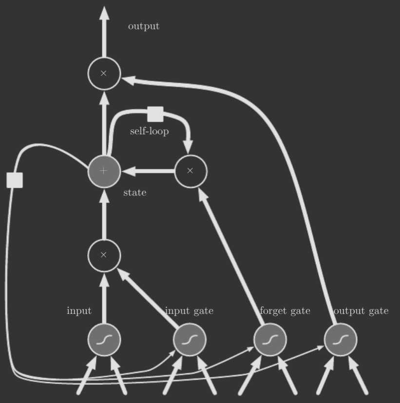
The key idea of the LSTM cell is its modification of the weight of the self-loop to be conditioned on the context, in that it is controlled by another hidden unit. This allows dynamic changes in the time scale of the unit. Note that LSTM cells are effectively drop-in replacements for the units of an RNN.

In particular, for a state unit $s_{i}^{(t)}$, the self-loop weight is controlled by a forget gate unit $f_{i}^{(t)}$ that sets the weight to

where $\boldsymbol{x}^{(t)}$ is the current input vector and $\boldsymbol{h}^{9t}$ is the current hidden layer vector. Also, $\boldsymbol{b}^{f},\boldsymbol{U}^{f},\boldsymbol{W}^{f}$ are the biases, input weights, and recurrent weights for the forget gates.

In addition to the forget gate, there is an external input gate unit $g_{i}^{(t)}$, which controls the weighting of the inputs at time step $t$.

The internal state is thus represented by

Finally, there is an output gate $q_{i}^{(t)}$, which controls the strength of the hidden-to-output weight. In fact, this allows shutting off the output $h_{i}^{(t)}$ of an LSTM cell!

Other Gated RNNs

There are alternative designs for RNNs with gated units. In particular, the namesake for gated RNNs, whose units are called gated recurrent units, have the following structure

where $u_{i}^{(t)}$ is the update gate and $r_{i}^{(t)}$ is the reset gate, and

These gates can individually "ignore" parts of the state vector. The update gate chooses, for each dimension, to either copy it or completely ignore it (corresponding to the two saturating ends of the sigmoid). The reset gate choose with parts of the state are used to compute the next target state.

10.11 Optimization for Long-Term Dependencies

Clipping Gradients

As aforementioned in chapter 8, strongly nonlinear functions tend to have derivatives of extreme magnitude (very small or very large), inducing cliffs in the objective function "landscape." This is particularly apparent for RNNs, due to their computations over many time steps. The difficulty this introduces is that an gradient descent update on a cliff may send the parameters much farther away than desired, making training much harder. And, notably, the model may frequently end up on cliff faces due to excessively large steps.

Gradient clipping is a family of methods designed to reduce the impact of such cliff updates. For instance, one may "clip" the norm $\lVert \boldsymbol{g} \rVert$ of the gradient $\boldsymbol{g}$ before the parameter update

for some constant norm threshold $v$. Another method clips each element of the gradient eventually. And, if the gradient explosion is severe enough that $\lVert \boldsymbol{g} \rVert$ is essentially NaN in software, even just a random step tends to work well.

Regularizing to Encourage Information Flow

The other consideration, of course, is vanishing gradients. LSTMs and gated units are effective for mitigating this, but another method is to "encourage information flow" by regularizing the gradient being back-propagated through the network to maintain its magnitude. Formally, we want

However, this approach is generally not as effective as the LSTM when there is an abundance of data.

10.12 Explicit Memory

Neural networks are great for storing implicit knowledge, i.e knowledge that is difficult to verbalize like "how to walk." However, they struggle to learn explicit knowledge—straightforward knowledge like simple facts. Memory networks are a type of neural network with special memory cells to store explicit knowledge.

These memory cells are accessed via an addressing mechanism, which originally required a supervision signal to direct the network on how to use it. However, the neural Turing machine (NTM) was introduced in 2014, based on a soft attention mechanism, to allow access without explicit supervision. However, it's difficult to optimize functions that produce exact integer addresses; instead, NTMs read/write to multiple memory cells simultaneously, reading weighted averages of many cells and modifying multiple cells by different amounts. The coefficients are typically chosen via a softmax function to select only a small number of cells, which also allows gradient descent to be performed on the functions controlling memory access.

The memory cells also typically contain vectors, rather than scalars, for two reasons.

• The computational cost of accessing memory is higher with the NTM (must produce a coefficient for every single cell), so reading a vector value from each cell somewhat offsets the cost.
• it enables content-based addressing, where the weight used to access a cell is a function of the cell's contents themselves. (e.g. a request like "Retrieve the sentence from X book starting with 'The quick brown fox...'"). This is in contrast to the traditional location-based addressing.