Chapter 9: Convolutional Networks

Convolutional neural networks or CNNs are a widely-popular type of neural network for processing data with a grid-like topology, such as time-series and images. The nomenclature is inspired by the operation employed by such networks: the convolution, a specialized linear operation. In fact, CNNs are just neural networks that use a convolution operation instead of a general matrix multiplication in at least one layer.

9.1 The Convolution Operation

The most general description of a convolution is an operation on two functions of real-valued argument.

Consider, for instance, a time-series of noisy measurements from some sensor, $x(t)$ . We can perform smoothing of the measurements by averaging together a window of past measurements; a weighted average, that favors more recent measurements, is most applicable. Let $w(a)$ be a weighting function that assigns a weight to a measurement according to its age $a$ . Then, the smoothed estimate is

s(t) \int x(a)w(t-a) \,\mathrm{d}a

This is a convolution, and is typically denoted with an asterisk.

s(t)=(x*w)(t)

In CNN terminology, the first argument $x$ is the input, the second argument $y$ is the kernel, and the output is the feature map. And, of course, for machine learning, we usually work with discrete rather than continuous convolutions, and often over multiple dimensions/axes. Note that, if the input becomes $n$ -dimensional, the kernel typically does too.

Convolution Commutativity

Convolutions are commutative. For an image $I$ and kernel $K$ , for instance,

(I*K)(i,j)=\sum_{m}\sum_{n}I(m,n)K(i-m,j-n)

is the same as

(K*I)(i,j)=\sum_{m}\sum_{n}I(i-m,j-n)K(m,n)

The latter is more frequently implemented in ML libraries.

Many networks also implement a related function, which is not the application of the commutative property of convolutions, known as cross-correlation.

(I*K)(i,j)=\sum_{m}\sum_{n}I(i+m,j+n)K(m,n)

The textbook refers to this as a convolution as well.

Notably, discrete convolution can be viewed as multiplication by a matrix! For univariate discrete convolution, the representing matrix must be a Toeplitz matrix. For two dimensions, it must be a doubly block circulant matrix. Moreover, the matrices are typically very sparse, as the kernel is usually much smaller than the input.

9.2 Motivation

Convolutions are based in three important ideas.

Sparse interactions
Parameter sharing
Equivariant representations

Moreover, they allow working with inputs of variable size.

Sparse Interactions

Also known as sparse connectivity or sparse weights. With a kernel much smaller than the input, much fewer parameters must be stored. Additionally, these effects compound exponentially through the layers of the network.

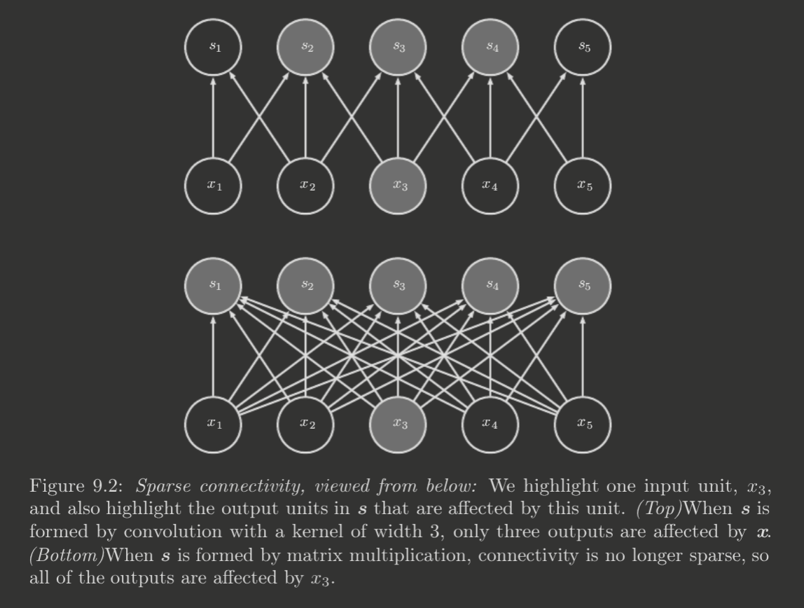
This greatly improves computational efficiency.

Parameter Sharing

Also known as tied weights. Parameter sharing, as aforementioned, refers to the use of an individual parameters multiple times in a model. In CNNs, each element of a kernel is used at (excluding some boundary positions) every position of the input.

This greatly improves memory requirements and statistical efficiency.

Equivariance

CNNs' particular application of parameter sharing grants the property of equivariance to translation. Formally, $f(x)$ is equivariant to $g(x)$ if $f(g(x))=g(f(x))$ . For CNNs, if $g$ is any translation function, then the convolution function $f$ is equivariant to $g$ .

This is useful for CNNs because of the type of data they process; they should be able to recognize the same patterns across time, for one-dimensional time series data, and across space, for two-dimensional images. Note, however, that convolutions are not equivariant to other types of transformations like rotations or dilations; these require further treatment.

9.3 Pooling

A typical layer of a CNN consists of three stages.

Convolution stage: layer performs convolutions in parallel $\to$ linear activations
Detector stage: nonlinear activation function applied (e.g. ReLU)
Pooling stage: pooling function applied

A pooling function essentially calculates some aggregate statistic of several outputs. For instance, the max pooling function returns the maximum output within a rectangular neighborhood. Pooling, in general, is helpful in promoting invariance to small translations in the input, and may be interpreted as an infinitely strong prior imposing this invariance. When correct, it increases statistical efficiency. Notably, pooling over separately parameterized convolutions can learn which transformations to develop invariance to.

Since pooling summarizes a neighborhood with one value, it's possible to space out pooling regions by $k$ units, rather than just $1$ . This helps improve computational efficiency, as it reduces the number of inputs into the next layer by a factor of $k$ .`

In fact, spaced pooling is an essential technique for handling variable size inputs—by varying the offset between pooling regions according to the input size, one may ensure the next layer receives the same number of summary statistics.

9.4 Convolution and Pooling as an Infinitely Strong Prior

A convolutional network can be interpreted as a fully connected network, except with an infinitely strong prior that requires the weights for each hidden unit to be identical to that of its neighbor, but shifted in space. Moreover, the prior mandates that all weights besides the receptive field assigned to that hidden unit must be $0$ . In other words, convolutions express an infinitely strong prior that the learned function contains only local interactions and is equivariant to translation.

9.5 Variants of the Basic Convolution Function

The convolution of machine learning differs from the standard discrete convolution operation of mathematics.

A convolution typically refers to the application of a convolution many times in parallel, in essence we are "convolving" the kernel across many locations.
The input is usually not a grid of real values, either; it is typically vector-valued. For instance, with images, the color channels induce a 3D tensor shape for the input and output of the convolution.

Downsampling is a technique to reduce the computational cost of the network, and functions by sampling only every $s$ pixels in each direction, for some stride $s$ . This does, of course, decrease the granularity of the layer.

Zero padding implicitly extends the width of the input tensor $\mathsf{V}$ ; otherwise, the representation width would shrink by at least one pixel every layer (since the pooling stage aggregates across multiple units). There are three important special cases of zero padding.

Valid convolution: no zero padding $\to$ limits number of convolutional layers
Same convolution: enough zero padding added to keep $\lvert \text{input} \rvert=\lvert \text{output} \rvert$ $\to$ no limit to layers, but input pixels near border are underrepresented
Full convolution: enough zero padding added to visit each pixel $k$ times in each direction (where $k$ is the kernel size in that direction) $\to$ output border pixels are influenced by fewer pixels than the center, makes learning the kernel difficult.

Typically the optimal amount of zero padding is between "valid" and "same" convolution.

Other times, locally connected layers are desired. In essence, a locally connected layer is a convolution layer without parameter sharing, and is thus sometimes called an unshared convolution. Meanwhile, tiled convolution is a compromise between a convolutional and locally connected layer, in which a set of kernels is learned that are rotated through (e.g. round robin style). Below demonstrates locally connected layers, tiled convolution, and standard convolution, respectively.

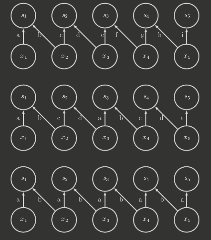
Locally connected and tiled convolutional layers, in contrast to convolutional layers, may learn invariance to transformations that are not just translations.

Bias

For locally connected layers, units are typically given their own bias. For tiled and standard convolutions, biases are usually shared.

9.6 Structured Outputs

Convolutional nets can also have output that is high-dimensional and structured.

example

Model output is a tensor $\mathsf{S}$ where $\mathsf{S}_{i,j,k}$ is the probability that pixel $(j,k)$ of the input belongs to class $i$ .

One issue, however, with such structured-output nets, is the comparatively small size of the output layer. This typically is induced by the large stride of some pooling layers; thus, it's sometimes desirable to avoid pooling or reduce stride size.

9.7 Data Types

The input data into a convolutional net typically consists of several channels at each point in space/time. For CNNs, it can also handle input data that has variable size, by scaling the pooling regions according to the input size.

9.8 Efficient Convolution Algorithms

Some kernels, of dimension $d$ , may be expressed as an outer product of $d$ vectors—these are separable kernels, and leads naturally into an optimization for naive convolution that performs $d$ outer products, i.e. $O(wd)$ time complexity, and requires a space complexity of $O(wd)$ as well. This replaces the $O(w^{d})$ time and space complexity of naive convolutions.

9.9 Random or Unsupervised Features

The most computationally expensive portion of CNN training is the (gradient descent) learning of features. Instead, some strategies learn the convolution kernels without supervised training; there are three main methods.

Initialize randomly
Design manually
Learn with unsupervised criterion

Random filters, in fact, work surprisingly well; thus, it's common to quickly test different CNN architectures by training just the last layer and evaluating performance.

Another approach is to learn the features without full forward and back-propagation—greedy layer-wise pretraining. CNNs take this further by training each layer on a small patch of the input at a time.

However, most modern CNNs are trained with the full supervised training process.

9.10 The Neuroscientific Basis for Convolutional Networks

Left out.

9.11 Convolutional Networks and the History of Deep Learning

Left out.