Chapter 8: Optimization for Training Deep Models

8.1 Learning vs. Pure Optimization

For a machine learning problem, there exists some performance measure $P$ that must be optimized; however, it's typically defined with respect to the test dataset (e.g. generalization error), and may be intractable to optimize. Thus, ML optimizes $P$ indirectly, minimizing a different but related cost function $J(\boldsymbol{\theta})$ and presuming that such a procedure will help optimize $P$ .

The cost function may usually be written as some average over the training set, such as

J(\boldsymbol{\theta})=\mathbb{E}_{(\boldsymbol{x},\mathrm{y})\sim \hat{p}_{\text{data}}}L(f(\boldsymbol{x};\boldsymbol{\theta}),y)

where $L$ is the loss function, $f(\boldsymbol{x};\boldsymbol{\theta})$ is the model's predicted output for input $\boldsymbol{x}$ , and $\hat{p}_{\text{data}}$ is the empirical distribution (training data).

Of course, it is preferable to actually minimize the objective function with respect to the true data generating distribution $p_{\text{data}}$ ; however, as aforementioned, this is inherently not possible.

J^{*}(\boldsymbol{\theta})=\mathbb{E}_{(\boldsymbol{x},\mathrm{y})\sim p_{\text{data}}}L(f(\boldsymbol{x};\boldsymbol{\theta}),y)

Empirical Risk Minimization

The goal of the model is to minimize the expected generalization error $J^{*}(\boldsymbol{\theta})$ . This is also known as the risk. With knowledge of the true distribution $p_{\text{data}}$ , risk minimization becomes a traditional optimization problem. But, with only a training set of samples, it becomes a machine learning problem.

The simplest approach, of course, is to minimize the empirical risk—the risk with respect to the empirical distribution/training set.

\mathbb{E}_{\boldsymbol{x},\mathrm{y}\sim \hat{p}_{\text{data}}(\boldsymbol{x},y)}[L(f(\boldsymbol{x};\boldsymbol{\theta}),y)]=\frac{1}{m}\sum_{i=1}^{m} L(f(\boldsymbol{x}^{(i)};\boldsymbol{\theta}),y^{(i)})

This is aptly termed empirical risk minimization, and this sort of method is very similar to traditional optimization—after all, we are now just applying optimization to a related quantity, the empirical risk, in hopes of reducing risk itself.

As discussed previously, though, this training approach tends to cause overfitting. Moreover, empirical risk minimization is not necessarily possible in all problems, considering some loss functions' tendencies to have zero/undefined derivatives (e.g. $0$ - $1$ loss).

Surrogate Loss Functions and Early Stopping

A surrogate loss function is a proxy loss function that is optimized in place of another loss function that is intractable to optimize. For instance, in classification, the negative log-likelihood of the correct class is often the surrogate for $0$ - $1$ loss.

Importantly, machine learning algorithms typically minimize a surrogate loss function but halts when a convergence criterion based on early stopping is satisfied; thus, they do not typically reach a local minimum. This is in direct contrast to a pure optimization setting, which stops only once the gradient vanishes.

Batch and Minibatch Algorithm

Additionally, ML algorithms, unlike pure optimization algorithms, typically have an objective function that decomposes as a sum over all training examples. However, computing it is expensive—in practice, it's approximated by randomly sampling a subset of training examples.

There a couple important motivations for this random sampling approach.

The standard error of the mean estimated from $n$ samples is $\frac{\sigma}{\sqrt{ n }}$ . This decreases sublinearly in $n$ ; therefore, optimization algorithms often converge much faster (in terms of total computation) with rapid, yet slightly more inaccurate estimates of the gradient.
There is typically a lot of redundancy in the training examples; not necessarily perfect duplicates, but examples that essentially encode very similar information.

Optimization algorithms that use the entire training set are batch or deterministic gradient methods. Those that use only a single example at a time are stochastic or online methods. The in-between, and more commonly used in deep learning, are minibatch or minibatch stochastic methods. They are frequently called simply stochastic, nowadays.

Why minibatch?

Sublinear returns for larger batch sizes
Multicore architectures are underutilized by extremely small batches $\to$ some minimum batch size
Parallel processing of batch of size $n$ scales memory linearly in $n$ .
Hardware performance improves for certain batch sizes (power of 2)
Small batches offer a regularization effect

warning

Minibatches must be sampled randomly (shuffling the dataset once before training is typically sufficient). Otherwise, this risks a biased estimate of the gradient.

Interestingly enough, minibatch stochastic gradient descent approximately follows the gradient of the true generalization error (provided examples are not repeated). The mathematical derivation of this is left out for brevity.

8.2 Challenges in Neural Network Optimization

Ill-Conditioning

Recall the condition number of the Hessian matrix $\boldsymbol{H}$ . This is believed to affect SGD when the model parameters find a region where even small steps increase the cost function. Recall the second-order approximation of the cost function. For a gradient descent step of $-\epsilon \boldsymbol{g}$ , it predicts a change to the cost of

\frac{1}{2}\epsilon^{2}\boldsymbol{g}^{\top}\boldsymbol{H}\boldsymbol{g}-\epsilon \boldsymbol{g}^{\top}\boldsymbol{g}

Ill-conditioning of the Hessian matrix becomes an issue when $\frac{1}{2}\epsilon^{2}\boldsymbol{g}^{\top}\boldsymbol{H}g^{\top}>\epsilon \boldsymbol{g}^{\top}\boldsymbol{g}$ .
To detect when ill-conditioning becomes detrimental, it's sufficient to monitor $\boldsymbol{g}^{\top}\boldsymbol{g}$ and $\boldsymbol{g}^{\top}\boldsymbol{H}\boldsymbol{g}$ during training.

Local Minima

Convex optimization enjoys the benefit that any local minimum is a global minimum as well. Therefore, it reduces an optimization problem to finding a local minimum.

With non-convex functions like neural networks, there may be many local minima that are not globally optimal. However, in practice, this is not a problem—most local minima for sufficiently large neural networks tend to have acceptably low costs.

To clarify if local minima is the issue behind a neural network, it helps to track the gradient during training. If the gradient's norm does not vanish, it's likely not the responsibility of suboptimal local minima. If it does vanish, it may be the fault of local minima; however, many other structures that are not local minima have small gradients, as we will see in the next section.

Plateaus, Saddle Points, and Other Flat Regions

Recall that a saddle point is associated with a Hessian matrix with both positive and negative eigenvalues, and may be interpreted as a local minimum along at least one cross section, and a local maximum along at lest one other cross section.

Random functions typically have many local minima in low dimensions, but have many more saddle points as dimensions grow—in fact, the ratio grows exponentially in $n$ for a function $f:\mathbb{R}^{n}\to \mathbb{R}$ . This can be intuitively explained by imagining each Hessian's eigenvalue as being determined by tossing a coin—the probability of a positive/negative definite matrix (non saddle point) would be $\frac{1}{2^{n-1}}$ .

An interesting property of many random functions, though, is that the eigenvalues of the Hessian are more likely to be positive in regions of lower cost. Intuitively, this is because it's more likely that, for critical points, the point is a local minima along more cross sections, considering the low cost. Therefore, in low cost regions, local regions become much more likely.

So, how do saddle points impact training, then? For first-order, gradient-based optimization, empirical evidence suggests they can frequently escape saddle points. However, for second-order techniques like Newton's method, which directly seek out a critical point—saddle points prove an issue as it may jump directly to a saddle point.

There are also other points with zero gradient, or very flat regions in the parameter space. Second-order optimization problems struggle more with zero gradient points, while flat regions pose a problem for all numerical optimization algorithms.

Cliffs and Exploding Gradients

Deep neural networks can often have extremely steep regions in parameter space—cliffs. This is a problem for gradient descent, as a small step may inadvertently change parameters substantially. They usually arise from the multiplication of large weights.

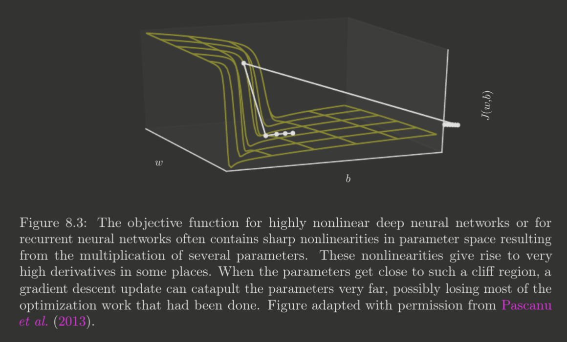
We describe techniques like gradient clipping later, in Chapter 10, for dealing with such regions, as they most prominently appear for recurrent neural networks.

Long-Term Dependencies

Sometimes, a neural network can be too deep. Recurrent networks, for instance, can generate extremely deep computational graphs (Chapter 10). Consider, for instance, a network that multiplies by a matrix $\boldsymbol{W}$ for $t$ steps. Given the eigendecomposition $\boldsymbol{W}=\boldsymbol{V}\text{diag}(\boldsymbol{\lambda})\boldsymbol{V}^{-1}$ , we deduce

\boldsymbol{W}^{t}=\boldsymbol{V}\text{diag}(\boldsymbol{\lambda})^{t}\boldsymbol{V}^{-1}

which tells us that any eigenvalues $\lambda_{i}>1$ will explode in magnitude and any $\lambda_{i}<1$ will vanish in magnitude. As gradients propagated through the graph are scaled according to $\text{diag}(\boldsymbol{\lambda})^{t}$ , this leads to the famous vanishing and exploding gradient problem. Vanishing gradients make learning slow, as parameters take extremely small steps, while exploding gradients (e.g. cliff structures) cause high learning instability.

We discuss techniques for treating these issues later in Chapter 10.

Inexact Gradients

Most optimization algorithms assume knowledge of an exact gradient or Hessian matrix. However, this is typically not the case—SGD, for instance, has only an estimate of the gradient. In other cases, the objective function being minimized may even be intractable, and thus must be approximated. There are various techniques designed to account for imperfect estimates... which the book does not expand on D:

Poor Correspondence between Local and Global Structure

There may be situations where the locally optimal direction of improvement does not correspond to eventual regions of sufficiently lower cost. The book notes that this is an active area of research, but that choosing a good initial point can help mitigate this problem sometimes.

Theoretical Limits of Optimization

Little impact on their use in practice.

8.3 Basic Algorithms

Stochastic Gradient Descent

Reference section 5.9 for a review of SGD. Previously, we described SGD in the context of a fixed learning rate $\epsilon$ . In practice, $\epsilon$ must be decreased over time, so we now use $\epsilon_{k}$ to denote the learning rate at iteration $k$ . This is because the SGD, as a random-sample gradient estimator, introduces a source of noise that does not vanish even when arriving at a minimum. Thus, to guarantee convergence of SGD, the learning rate must satisfy

\sum_{k=1}^{\infty} \epsilon_{k}=\infty

and

\sum_{k=1}^{\infty} \epsilon_{k}^{2}<\infty

In practice, a decay scheme such as

\epsilon_{k}=(1-\alpha)\epsilon_{0}+\alpha\epsilon_{\tau}

is used, where $\alpha=\frac{k}{\tau}$ . In other words, this decays $\epsilon$ linearly every iteration until iteration $\tau$ , at which point $\epsilon$ is left constant.

Notably, $\epsilon_{0}$ , $\epsilon_{\tau}$ , $\tau$ must be chosen beforehand. Usually $\epsilon_{\tau}\approx 0.01\epsilon_{0}$ . $\tau$ is typically set to the number of iterations to make a few hundred passes through the training set. $\epsilon_{0}$ , however, should be carefully tuned according to model performance.

The most important property of SGD is that the computation time per update does not grow with training set size, allowing convergence with extremely large datasets. Convergence rate of optimization algorithms may be measured with the excess error

J(\boldsymbol{\theta})-\min _{2\boldsymbol{t}}J(\boldsymbol{\theta})

or the difference between the current cost and the minimum possible cost. Batch gradient descent does, in theory, have better convergence rate; however, the computational advantage of SGD outweighs its slow asymptotic convergence.

Momentum

SGD, despite its strengths, can be slow to learn when faced with a parameter space with

High curvature
Small gradients
Noisy gradients

The momentum algorithm introduces a variable $\boldsymbol{v}$ that represents the current velocity of the parameters. This allows the changes applied in previous iterations to continue to affect the parameters in the current iteration. Momentum is inspired, of course, by the concept of momentum in physics and Newton's First Law—an object in motion stays in motion! However, conservation of momentum is not preserved for optimization; instead, the velocity exponentially decays over time, according to some hyperparameter $\alpha \in[0,1)$ , to ensure more recent gradients take higher precedence. (In physics terminology, one may imagine this to be viscous drag in some resistant medium). Formally,

\begin{align*} \boldsymbol{v}&\leftarrow\alpha \boldsymbol{v}-\epsilon \nabla_{\boldsymbol{\theta}}\left( \frac{1}{m}\sum_{i=1}^{m} L(\boldsymbol{f}(\boldsymbol{x}^{(i)};\boldsymbol{\theta}),\boldsymbol{y}^{(i)}) \right) \\ \boldsymbol{\theta}&\leftarrow\boldsymbol{\theta}+\boldsymbol{v} \end{align*}

Note that larger $\alpha$ corresponds to a greater conservation of momentum, i.e. previous gradients have more influence.

The most interesting effect of the momentum algorithm, of course, is the speed increase. Consider a sequence of the gradients that are all the same, i.e. they are all $\boldsymbol{g}$ . Then, the algorithm will actually accelerate in the direction of $-\boldsymbol{g}$ until it reaches a terminal velocity, where each step changes the parameters by

\frac{\epsilon \lVert \boldsymbol{g} \rVert }{1-\alpha}

Like the learning rate, $\alpha$ may also be adapted over time, though less important. Typically, it starts small and increases with more iterations.

Nesterov Momentum

Nesterov momentum is a variant of the original momentum algorithm inspired by Nesterov's accelerated gradient method. The new updates rules are

\begin{align*} \boldsymbol{v}&\leftarrow\alpha \boldsymbol{v}-\epsilon \nabla_{\boldsymbol{\theta}}\left[ \frac{1}{m}\sum_{i=1}^{m} L(\boldsymbol{f}(\boldsymbol{x}^{(i)};\boldsymbol{\theta}+\alpha \boldsymbol{v}),\boldsymbol{y}^{(i)}) \right] \\ \theta&\leftarrow\boldsymbol{\theta}+\boldsymbol{v} \end{align*}

The difference between Nesterov and traditional momentum is the $\boldsymbol{\theta}+\alpha \boldsymbol{v}$ term in $\boldsymbol{f}(\boldsymbol{x}^{(i)};\boldsymbol{\theta}+\alpha \boldsymbol{v})$ . In other words, the gradient is evaluated at the point after the current velocity is applied, and may be interpreted as a correction factor that takes into account the effect of the previous gradients when calculating the gradient.

8.4 Parameter Initialization Strategies

Deep learning is actually strongly affected by parameter initialization, as they significantly influence learning stability, convergence rate, final cost, and generalization error. Despite this, modern initialization strategies are generally simple and heuristic, as there is no clear solution to initialization.

The only understood idea is that the parameter initialization should intend to create asymmetry between units—otherwise, a deterministic learning algorithm and cost function will result in the same updates for both units.

This property motivates random initialization—this usually provides sufficiently good performance for low computational cost. Note, though, that this primarily applies to weights; other parameters, like biases, are chosen heuristically.

Typically, random initialization draws from a uniform or Gaussian distribution. One must be careful, though, to set the scale of the distribution carefully: while larger units create greater asymmetry, they can also cause exploding values, saturate units, and, in recurrent networks, induce chaos, extreme sensitivity to small input perturbations.

If possible, it's desirable to treat scale as a hyperparameter, and tune accordingly. One may also tune the sparsity of the parameter initialization. It's common to look for feedback in the range/standard deviations of activations/gradients; too small $\to$ increase scale.

For biases, while setting them to $0$ is actually sufficient, usually, we employ heuristic initialization sometimes.

Output units: bias for the output unit may want to represent some statistic of the output.
Saturation: ReLUs saturate at $0$ , so it's desirable to choose some small nonzero bias.
Gates: some units act as gates/switches that turn other units on/off—usually, we want to initialize these gates as "on" so it may learn. This is most applicable in Chapter 10, for gated recurrent units.

8.5 Algorithms with Adaptive Learning Rates

AdaGrad

AdaGrad uses an individual learning rate for each parameter, where parameter $i$ 's learning rate at time $t$ is proportional to a historical average, i.e.

\epsilon_{i}^{(t)} \propto \sqrt{ \frac{1}{\sum_{t'=1}^{t-1} (\epsilon_{i}^{(t')})^{2}} }

Parameters with larger gradients/greater curvature are assigned smaller learning rates. Empirically, however, it has been show that AdaGrad weights gradients from the beginning of training too heavily in non-convex settings.

RMSProp

RMSProp is AdaGrad except the summation average is changed to an exponentially decaying weighted moving average. It is frequently combined with Nesterov momentum, and has generally performed well.

Adam

The name Adam derives from "adaptive moments." It may be seen as a variant of RMSProp + momentum with a few distinctions.

Adam uses (exponentially weighted) momentum to estimate the first order moment (velocity) of the gradient.
Adam applies bias corrections to the estimates of the first-order moment (velocity) and the second-order moment (the moving average) that accounts for their initialization at the origin.

8.6 Approximate Second-Order Methods

Newton's Method

We briefly review Newton's method.

It it based on a second-order Taylor series approximation of $J(\boldsymbol{\theta})$ at some point $\boldsymbol{\theta}_{0}$

J(\boldsymbol{\theta})\approx J(\boldsymbol{\theta}_{0})+(\boldsymbol{\theta}-\theta_{0})^{\top}\nabla_{\boldsymbol{\theta}}J(\boldsymbol{\theta}_{0})+\frac{1}{2}(\boldsymbol{\theta}-\boldsymbol{\theta}_{0})^{\top}\boldsymbol{H}(\boldsymbol{\theta}-\boldsymbol{\theta}_{0})

where the Hessian $\boldsymbol{H}$ is evaluated at point $\boldsymbol{\theta}_{0}$ . Solving for the critical point provides the Newton parameter update rule

\boldsymbol{\theta}^{*}=\boldsymbol{\theta}_{0}-\boldsymbol{H}^{-1}\nabla_{\boldsymbol{\theta}}J(\boldsymbol{\theta}_{0})

For locally quadratic functions, Newton's method may jump directly to a minimum. For convex functions, the method may be iterated to perform second-order descent.

However, as noted in [[#Plateaus, Saddle Points, and Other Flat Regions|section 8.2]], Newton's method may fail when the function is non-convex, i.e. has critical non-minima like saddle points. When $\boldsymbol{H}$ is not positive definite, then Newton's method can result in suboptimal choices. Thus, the Hessian is frequently regularized; one strategy is to add a constant $\alpha$ along the Hessian's diagonal.

\boldsymbol{\theta}^{*}=\boldsymbol{\theta}_{0}-[\boldsymbol{H}+\alpha \boldsymbol{I}]^{-1}\nabla_{\boldsymbol{\theta}}f(\boldsymbol{\theta}_{0})

This works well provided light negative curvature.

Regardless, Newton's method is also impractical considering the computation of the inverse Hessian, an $O(k^{3})$ operation. Thus, further sections discuss how to use Newton's method without such computational burden.

Conjugate Gradients

Conjugate gradients is a method in which one iteratively descends conjugate directions—directions that do not undo progress made by previous steps—to avoid computing the inverse Hessian.

This is done by accounting for the previous direction $\boldsymbol{d}_{t-1}$ in the current direction.

\boldsymbol{d}_{t}=\nabla_{\boldsymbol{\theta}}J(\boldsymbol{\theta})+\beta_{t}\boldsymbol{d}_{t-1}

Where $\beta_{t}$ controls the contribution of $\boldsymbol{d}_{t-1}$ .

Two directions $\boldsymbol{d}_{t}$ and $\boldsymbol{d}_{t-1}$ are conjugate if

\boldsymbol{d}_{t}^{\top}\boldsymbol{H}\boldsymbol{d}_{t-1}=0

Of course, we should not calculate the Hessian; however, there exist methods of efficiently computing $\beta_{t}$ without directly computing $\boldsymbol{H}$ . For instance, the Fletcher-Reeves:

\beta_{t}= \frac{\nabla_{\boldsymbol{\theta}}J(\boldsymbol{\theta})_{t}^{\top}\nabla_{\boldsymbol{\theta}}J(\boldsymbol{\theta}_{t})}{\nabla_{\theta}J(\boldsymbol{\theta}_{t-1})^{\top}\nabla_{\boldsymbol{\theta}}J(\boldsymbol{\theta}_{t-1})}

Note that conjugate gradients is applied with a line search for the minimum along the direction $\boldsymbol{d}_{t}$ . And, in nonlinear cases, it's necessary to sometimes reset the line search to use the unaltered gradient (i.e. not factoring in the previous direction) because the regular conjugate directions method no longer ensures that it does not undo progress by previous steps. Despite this, conjugate methods shows some positive results in deep learning.

BFGS

The Broyden-Fletcher-Goldfarb-Shanno algorithm approximates $\boldsymbol{H}^{-1}$ with a matrix $\boldsymbol{M}_{t}$ that is iteratively changed by low rank updates to more closely approximate $\boldsymbol{H}^{-1}$ . The parameter update transforms from

\boldsymbol{\theta}_{t+1}=\boldsymbol{\theta}_{t}-\boldsymbol{H}^{-1}\nabla_{\boldsymbol{\theta}}J(\boldsymbol{\theta}_{t})

\boldsymbol{\theta}_{t+1}=\boldsymbol{\theta}_{t}+\epsilon^{*}\boldsymbol{p}_{t}

where $\boldsymbol{p}_{t}=\boldsymbol{M}_{t}\boldsymbol{g}_{t}$ . (And $\boldsymbol{g}_{t}=\nabla_{\boldsymbol{\theta}}J(\boldsymbol{\theta}_{0})$ ).

Like conjugate gradients, BFGS also uses a line search in the direction of $\boldsymbol{p}^{t}$ to determine the best $\epsilon^{*}$ ; however, it is not as dependent on the line search as conjugate gradients, and may spend less time.

However, the most prominent issue with BFGS is that it must store an approximation of the inverse Hessian in memory— $O(n^{2})$ , impractical for modern deep learning models. Limited Memory BFGS (L-BFGS) tries to mitigate this issue by simply assuming $\boldsymbol{M}_{t-1}$ is the identity matrix, for each step. In other words, it no longer iteratively updates $\boldsymbol{M}$ , but just provides a rough approximation at each step. A better approach, however, that generalizes L-BFGS, is to store some (constant number) of vectors describing $M_{t-1}$ . This costs only $O(n)$ memory each step, and provides better performance.

8.7 Optimization Strategies and Meta-Algorithms

This section, we discuss optimization techniques that are general templates or subroutines applicable to many algorithms.

Batch Normalization

Batch normalization intends to address higher-order effects, especially those that arise in deep neural networks.

Consider a deep neural network with one unit per layer and no activation function. The output is

\hat{y}=xw_{1}w_{2}\dots w_{l}

where $l$ is the depth. The change to $\hat{y}$ from the gradient update $\boldsymbol{w}\leftarrow \boldsymbol{w}-\epsilon \boldsymbol{g}$ is

\hat{y}=x(w_{1}-\epsilon g_{1})(w_{2}-\epsilon g_{2})\dots (w_{l}-\epsilon g_{l})

Evidently, this will produce many higher order terms—some of which may be exponentially large with just a few layers with weights $>1$ . In other words, the interactions between layers can produce substantial higher-order interactions that are amplified as depth increases.

Batch normalization tackles this problem by individually normalizing layers. Consider a minibatch of activations of a layer to normalize, $\boldsymbol{H}$ , where the activations of each example correspond to a row of $\boldsymbol{H}$ . During training, we replace $\boldsymbol{H}$ with

\boldsymbol{H}'= \frac{\boldsymbol{H}-\boldsymbol{\mu}}{\boldsymbol{\sigma}}

where $\boldsymbol{\mu}$ is a vector of the mean activation of each unit and $\boldsymbol{\sigma}$ is a vector of the standard deviation of each unit, i.e.

\begin{align*} \boldsymbol{\mu}&=\frac{1}{m}\sum_{i}\boldsymbol{H}_{i,:} \\ \boldsymbol{\sigma}&=\sqrt{ \delta+\frac{1}{m}\sum_{i}(\boldsymbol{H}-\boldsymbol{\mu})_{i}^{2} } \end{align*}

where $\delta$ is a small positive value to avoid $\sigma=0$ creating undefined gradients.

At inference time, $\boldsymbol{\mu}$ and $\boldsymbol{\sigma}$ are replaced by running averages collected during training time.

In short, batch normalization normalizes the next layer's inputs, or the current layer's outputs. This ensures that small amplifications do not explode into massive higher-order effects for later layers. Critically, this transformation is differentiable, and is thus included in backpropagation. This ensures the gradient never tries to just increase standard deviation or mean of $h_{i}$ to lower cost.

Formally, batch normalization solves the internal covariate shift problem, which generally describes the changes in the means and standard deviations affecting the inputs to the networks' inner layers (i.e. the activations of previous layers).

Notably, modern batch initialization actually replaces $\boldsymbol{H}$ with $\boldsymbol{\gamma} \boldsymbol{H}'+\boldsymbol{\beta}$ for learned parameters $\boldsymbol{\gamma}$ and $\boldsymbol{\beta}$ that represent the mean and standard deviation of the activations. This is because normalizing the mean and standard deviation reduces the expressiveness of the layer. In short, this approach allows the model to choose parameters $\boldsymbol{\gamma},\boldsymbol{\beta}$ for the mean and standard deviation when they actually do perform better than the normalized mean activations.

Isn't this useless? Doesn't this just unnormalize the distribution?

Yes, it does allow the model to unnormalize the distribution. However, the critical idea is that the mean of $\boldsymbol{\gamma}\boldsymbol{H}'+\boldsymbol{\beta}$ is determined solely by $\boldsymbol{\beta}$ , which is actually easier for gradient descent to learn. Otherwise, the mean is parameterized by complex, higher-order interactions between previous layers.

Coordinate Descent

Coordinate descent minimizes $f(\boldsymbol{x})$ by iteratively optimizing with respect to an individual variable, i.e. minimize w.r.t $x_{i}$ , then $x_{j}$ , etc., cycling through the variables if necessary. Block coordinate descent is a generalization that, in each step, optimizes w.r.t a subset of the variables simultaneously. "Coordinate descent" is often used to refer to either.

This methodology applies when the different variables can be clearly separated into groups. Consider the cost function

J(\boldsymbol{H},\boldsymbol{W})=\sum_{i,j}\lvert H_{i,j} \rvert +\sum_{i,j}(\boldsymbol{X}-\boldsymbol{W}^{\top}\boldsymbol{H})^{2}_{i,j}

which describes a learning problem sparse coding, with a goal of finding a weight matrix $\boldsymbol{W}$ that can essentially reverse a matrix of activation values $\boldsymbol{H}$ to reconstruct the training set. (Essentially, find a way to encode the training set with a sparse representation).

$J$ is not convex. However, we can divide the inputs into the weight matrix parameters $\boldsymbol{W}$ and the "code" representations $\boldsymbol{H}$ , and minimization w.r.t to each individually is convex.

Polyak Averaging

Polyak averaging essentially averages together the points in parameter space visited by an optimization algorithm to produce a final parameterization. For instance, if $\hat{\boldsymbol{\theta}}$ is the final parameterization after the $t$ th iteration,

\hat{\boldsymbol{\theta}}^{(t)}=\frac{1}{t}\sum_{i}\boldsymbol{\theta}^{(i)}

the above algorithm performs well, empirically, on convex problems for neural networks. The intuition is that an optimization algorithm may traverse across a valley several times without reaching the bottom, and so averaging the past parameterization likely produces a point closer to the bottom of the valley.

In non-convex problems, the structure is not so simple. However, an exponentially decaying running average remains applicable

\hat{\boldsymbol{\theta}}^{(t)}=\alpha\hat{\boldsymbol{\theta}}^{(t-1)}+(1-\alpha)\boldsymbol{\theta}^{(t)}

Supervised Pretraining

Any strategy that involves training simple models on simple tasks before training the desired model on the desired task is known as pretraining.

Greedy algorithms, for instance, break a problem into components, optimize each component, and then combine them to yield a solution. The final solution, while not optimal, is generally acceptable and computationally inexpensive. They may also be followed by a fine-tuning stage; in fact, initializing an optimization algorithm for the full problem with a greedy solution may improve convergence rate and solution cost.

In particular, we discuss greedy supervised pretraining—algorithms that break supervised learning problems into simpler supervised learning problems.

The original invention of greedy supervised pretraining involved several stages that trained only a subset of the layers in the total neural network. Other variants slowly add more layers to training, or train each layer individually using the outputs of previous layers as the input.

The original paper also hypothesized that greedy supervised pretraining provides benefits because it provides better guidance for intermediate levels of deep networks. Practically speaking, it may benefit both optimization and generalization.

This extends to the concept of transfer learning, in which a network that is pretrained on one set of tasks is used to initialize another network trained on a different set of tasks. Another related idea is FitNets, in which a small network is first trained as a teacher, and then a larger network is trained as a student by predicting both the output and the activations of the middle layers of the teacher network.

Designing Models to Aid Optimization

Many advancements in the optimization of deep models have been a result of designing models to be easier to optimize. In fact, in principle, it is more important to choose a model family that is easy to optimize than to use a powerful optimization algorithm.

Consider, for instance, the linear transformations inherent to neural networks, and the ease of differentiability (and also linearity) of activation functions. More recent ideas like skip connections (connecting non-adjacent layers) and auxiliary heads (copies of the output attached to hidden layers) also all intend to make training easier.

Continuation Methods and Curriculum Learning

As aforementioned, one issue in optimization is when local updates do not necessarily reflect moves toward globally low cost regions. Most solutions try to initialize parameters such that local updates do reflect global structure.

Continuation methods construct a series of objective functions $\{ J^{(0)},\dots,J^{(n)} \}$ over the same parameters that are designed to be increasing difficult/less well-behaved. The objective functions are then optimized incrementally in order, where $J^{(i-1)}$ 's final point is used for $J^{(i)}$ 's initial point. The idea is that each objective function will likely start with a good initial point, and that more well-behaved functions are more likely to have local updates reflect global structure.

Traditional continuation methods were typically based on smoothing the objective function—the idea was that non-convex functions become approximately convex when blurred, preserving global minima but "blurring away" local minima. However, it has several issues.

High computational cost
Blurred function may not be convex
Minimum of blurred function is not necessarily the global minimum

Also, note that continuation methods were originally designed to avoid local minima; this is no longer believed to be a predominant issue in neural network optimization, and thus their purpose has changed.

One specific continuation method, curriculum learning or shaping, attempts to train a model by learning simpler concepts first (training on simpler examples), before progressing to more complex concepts. The curriculum may be deterministic or stochastic, i.e. random mix of simple/complex examples with the proportion of complex examples increasing during training.