Chapter 7: Regularization for Deep Learning

As aforementioned, regularization is the study of how to train models that generalize well to unseen inputs. For deep learning, most regularization strategies are based on regularizing estimators, typically by sacrificing bias (increasing bias) to reduce variance. In other words, preventing overfitting.

7.1 Parameter Norm Penalties

The simplest form of regularization is a parameter norm penalty $\Omega(\boldsymbol{\theta})$, added to the objective function $J$ to produce the regularized objective function $\tilde{J}$.

Note that $\alpha \in[0,\infty)$ is a hyperparameter that weights the contribution of the penalty term $\Omega$. Larger $\alpha$ induces grater regularization. This section, we'll discuss the choice of the parameter norm $\Omega$ and its effects.

$L^{2}$ Regularization

We begin with the simplest parameter norm penalty: $L^{2}$ or weight decay. It's also known as ridge regression or Tikhonov regularization, and involves adding a regularization term $\Omega(\boldsymbol{\theta})=\frac{1}{2}\lVert \boldsymbol{w} \rVert^{2}_{2}$.

The new cost function gradient is then

And the gradient step is

In other words, the weight decay term induces the gradient descent to shrink the previous weight vector by a constant factor on each step. So, what happens across the entirety of training?

We first simply analysis by making a quadratic approximation (Taylor series) of the (original) objective function in the neighborhood of the cost-minimizing weights:

where $\boldsymbol{H}$ is the Hessian matrix of $J$ with respect to $\boldsymbol{w}$ evaluated at $\boldsymbol{w}^{*}=\arg\min_{\boldsymbol{w}}J(\boldsymbol{w})$, the cost-minimizing weights.

Naturally, the minimum of $\hat{J}$ occurs when its gradient

is $\mathbf{0}$.

Now, consider adding the weight decay back. Now, the gradient becomes

where $\tilde{\boldsymbol{w}}$ represents the minimum of the regularized version of the approximation $\hat{J}$. Equating to $0$ and solving for $\tilde{\boldsymbol{w}}$, we derive

Note that $\lim_{ \alpha \to 0 }\tilde{\boldsymbol{w}}=\boldsymbol{w}^{*}$. But what about when $\alpha$ grows?

$\boldsymbol{H}$ is real and symmetric, therefore we can eigendecompose it. This allows deriving

In words, this means that weight decay effectively rescales $\boldsymbol{w}^{*}$ along the axes defined by the eigenvectors of $\boldsymbol{H}$. Specifically, the component of $\boldsymbol{w}^{*}$ aligned with eigenvector $v_{i}$ of $\boldsymbol{H}$ is rescaled by a factor of $\frac{\lambda_{i}}{\lambda_{i}+\alpha}$. See section 2.7 if you're confused.

Thus, along directions where $\lambda_{i}\gg\alpha$, the regularization has minimal effect. In contrast, if $\lambda_{i}\ll\alpha$, these components will be shrunk significantly. A visualization is displayed below.

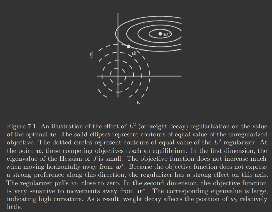
In other words, only directions that contribute substantially to reducing the cost function are preserved.

One can interpret its effects, for instance, on linear regression. Applying $L^{2}$ regularization changes the solution to

Note that the covariance matrix is $\frac{1}{m}\boldsymbol{X}^{\top}\boldsymbol{X}$. Thus, $L^{2}$ regularization, adding $\alpha$ to each element of the diagonal, appears to induce additional variance in the input (recall that $\mathrm{Cov}(X, X)=\mathrm{Var}(X)$) and thus shrink the weights for features whose covariance with the output target is comparatively small.

$L^{1}$ Regularization

Formally,

and

with gradient

Notably, the contribution of the regularization term no longer scales according to $w_{i}$; instead, it is either $-\alpha$ or $+\alpha$. This actually means that there are no clean algebraic solutions to quadratic approximations of $J(\boldsymbol{X},\boldsymbol{y};\boldsymbol{w})$, like there were for $L^{2}$ regularization.

We can still interpret the quadratic approximation, however. Again,

Given our limitations, we will assume the Hessian is diagonal with all positive elements. This holds if the data has been preprocessed to remove correlation between input features (e.g. preprocess with PCA). Thus, the approximation of our regularized objective function becomes

The analytical solution is

WLOG, let $w_{i}^{*}>0$ for all $i$. Consider if

• $w_{i}^{*}\leq \frac{\alpha}{H_{i,i}}$. Then, the optimal value of $w_{i}$ under regularization is $w_{i}=0$.
• $w_{i}^{*}> \frac{\alpha}{H_{i,i}}$. Then, the regularization simply shifts it towards zero by $\frac{\alpha}{H_{i,i}}$.

The behavior is similar with for $w_{i}^{*}<0$.

The notable aspect of $L^{1}$ regularization, as hinted above, is that it produces a sparse solution, as it zeroes some parameters. ($L^{2}$ regularization does not introduce sparsity; rescaling never zeroes a component). This is critical for tasks like feature selection, i.e. selecting a subset of the available features to be used as input. This is well known as LASSO (Least Absolute Shrinkage and Selection Operator) in the context of linear models.

7.2 Norm Penalties as Constrained Optimization

We previously alluded to the relation between norm penalties and the generalized Lagrange function used for constrained optimization. We now discuss this in more detail.

For instance, if we wanted to constraint $\Omega(\boldsymbol{\theta})<k\in \mathbb{R}$, we construct a generalized Lagrangian

With solution

Though, as mentioned in section 4.4, solving the problem requires learning/solving for both $\boldsymbol{\theta}$ and $\alpha$. Theoretically, it's possible to solve for the value of $k$ that corresponds to an $\alpha$; however, it varies depending on the objective function $J$ itself. Instead, we use $\alpha$ as a hyperparameter, and manually control it to roughly adjust the constraint region. Again, larger $\alpha$ strengthens the constraints, while smaller $\alpha$ weakens them.

Occasionally, however, explicit constraints are desired, i.e. we want to limit $\Omega(\boldsymbol{\theta})$ by a precisely chosen value of $k$. Rather than solving for the corresponding $\alpha$, this can be done by using SGD and then projecting $\boldsymbol{\theta}$ back to the nearest constraint-satisfying point. This explicit constraints and reprojection method is, at times, useful:

• Using penalties can result in non-convex optimization algorithms getting stuck in local minima
• Optimization algorithms with high learning rates can encounter positive feedback loops, which are unregulated without explicit constraints.

7.3 Regularization and Under-Constrained Problems

Regularization may even be necessary for a machine learning problem to be properly defined.

For instance, many linear models depend on inverting $\boldsymbol{X}^{\top}\boldsymbol{X}$, which may not be invertible. Thus, many use $\boldsymbol{X}^{\top}\boldsymbol{X}+\alpha \boldsymbol{I}$ instead, which is always invertible.

For underdetermined problems, learning algorithms may never converge; regularization can ensure convergence eventually occurs.

7.4 Dataset Augmentation

In practice, data is limited. One solution for this is the creation of fake data. Depending on the task, this may be straightforward!

Injecting noise into the input of a neural network is also data augmentation. Many tasks should be possible to solve even with small perturbations to the input. Noise injection also works for hidden units; dropout, which we discuss soon, can be interpreted as constructing new inputs by multiplying by noise.

7.5 Noise Robustness

As aforementioned, it's desirable for a model to be resistant to noise in the inputs. Beyond just injecting noise into the inputs, it's possible to achieve this by injecting noise into the weights. Adding small perturbations during training actually encourages parameters to tend to regions of parameter space that are flat, i.e. insensitive to small variations of weights. Refer to the book for the math behind this.

It's also possible to inject noise into the output targets. This is desirable because datasets frequently have some mistakes in the outputs. Label smoothing is one technique that regularizes a model with a softmax of $k$ different values by replacing hard $0,1$ classification targets with targets of $\frac{\epsilon}{k-1}$ and $1-\epsilon$, where we are assuming each category label $y$ is correct with probability $1-\epsilon$. This also helps encourage convergence for maximum likelihood learning.

7.6 Semi-Supervised Learning

In semi-supervised learning, we use both unlabeled examples from $P(\mathbf{x})$ and labeled examples from $P(\mathbf{x},\mathbf{y})$ to estimate $P(\mathbf{y}\mid \mathbf{x})$. The motivation is that the unsupervised part of the learning can hint towards how to group examples in representation space. In essence, you can think of the unsupervised part as performing the clustering, and the supervised part actually labeling the clusters.

It's not necessary to separate the unsupervised and supervised components, however. It's possible to construct models in which a generative/unsupervised model, either $P(\mathbf{x})$ or $P(\mathbf{x},\mathbf{y})$ shares parameters with a discriminative/supervised model of $P(\mathbf{y}\mid \mathbf{x})$. One may then minimize some function of the supervised criterion $-\log P(\mathbf{y}\mid \mathbf{x})$ and the unsupervised/generative criterion. In essence, the generative criterion expresses a prior about the supervised problem's solution; that the structures are connected in a way that may be captured via shared parametrization.

7.7 Multi-Task Learning

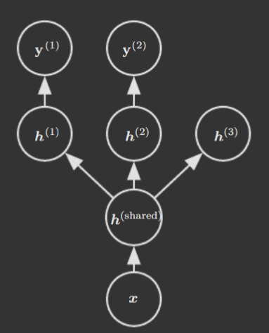
Multi-task learning involves using examples from several different tasks to improve generalization. A very common form of multi-task learning involves the different tasks sharing the same input $\mathbf{x}$ and some portion of the hidden layers $\boldsymbol{h}^{(\text{shared})}$ intended to capture some common factors—generic parameters. The other hidden layers (and output layer) are the task-specific parameters. Below shows an example architecture.

7.8 Early Stopping

When training large models with sufficient representational capacity to overfit, training error will typically continuously decrease, but validation error will begin increasing after enough iterations. Therefore, it's frequently (really, almost always) desirable to stop the gradient descent algorithm at some point, when the training error has become sufficiently small, to prevent overfitting.

The most common method for this is recording the validation error every time we see an improvement, and returning to the parameter values at the point in which the validation error is minimized. This is known as early stopping, and can be interpreted as an efficient hyperparameter selection algorithm where we treat the number of training steps as a hyperparameter.

Early stopping is popular for a couple reasons.

• No trial and error for number of training steps
• Easy to add without harming learning dynamics
• It acts as a regularizer

There are a couple considerations with early stopping, though. Early stopping requires a validation set; a common strategy is to perform two sets of training—one without the validation set that uses early stopping, and then one with all training data (i.e. validation set is now training data). There are two options for the second training procedure.

• Reset parameters, and retrain for the same number of steps as the first training, which early stopping determined to be optimal.
• Keep parameters, and continue training, but with all data. This avoids the cost of retraining, but is not well-behaved without a good guide for when to stop. Practically, the algorithm stops when the average loss function on the validation set falls below the loss at the end of early stopping.

Previously, we discussed how early stopping acts as a regularizer. Now, we formalize this notion, and show that early stopping essentially equates to $L^{2}$ regularization (for a simple linear model with quadratic error function trained by gradient descent).

As before, we make a quadratic approximation of the cost function $J$ in the neighborhood of the optimal weights $\boldsymbol{w}^{*}$.

And compute the gradient

Now, we consider how the parameters change during gradient descent. WLOG, assume $\boldsymbol{w}^{(0)}=\mathbf{0}$.

Rewriting with $\boldsymbol{H}$'s eigendecomposition and simplifying returns (plus some small assumptions)

While doing some rearrangement in the $L^{2}$ equation from [[7. Regularization for Deep Learning#$L {2}$ Regularization|section 7.1]] gives

Therefore, if hyperparameters $\epsilon,\alpha,\tau$ are chosen such that

$L^{2}$ regularization and early stopping are equivalent! In fact, one can conclude that $\tau \approx\frac{1}{\epsilon\alpha}$, provided the eigenvalues are sufficiently small.

Intuitively, this is because training learns the directions of high curvature first, and early stopping halts training before the model learns directions of low curvature. Of course, the equivalence only holds for a quadratic approximation of the objective function; however, the primary idea of this relationship generally holds.

7.9 Parameter Tying and Sharing

Frequently, we may want to express a prior that two models should be similar to each other. For instance, two models performing the same classification task with slightly different input distributions.

For this purpose, we can add a parameter norm penalty that ties the models' parameters to each other

for models $A$ and $B$. However, a more popular approach is actually to use constraints that force sets of parameters to be equal—this is parameter sharing. The primary advantage of this approach is that it reduces memory footprint—only a subset of the parameters, i.e. the unique shared set, need to be stored in memory.

7.10 Sparse Representations

Recall the $L^{1}$ regularization penalty, and how it encourages a sparse parameterization, i.e. encourages many weights to be $0$. Sparseness can also be encouraged in the representation of the data, i.e. in the hidden layers (e.g. a hidden layer with only a few active units). This can be implemented with a norm penalty on the representation:

where $\boldsymbol{h}$ represents a hidden layer(s). For sparsity, an $L^{1}$ penalty is typically useful; though other sparsity-encouraging penalties exist too.

Other approaches place a hard constraint on activation values instead. Orthogonal matching pursuit, for instance, seeks a representation $\boldsymbol{h}$ such that

where $\lVert \boldsymbol{h} \rVert_{0}$ denotes the number of nonzero entries of $\boldsymbol{h}$, i.e. it limits the number of active units in the layer to $<k$. The problem is tractable when $\boldsymbol{W}$ is constrained to be orthogonal, hence the nomenclature, and is often termed "OMP-$k$."

7.11 Bagging and Other Ensemble Methods

Bagging, or bootstrap aggregating, separately trains different models and then asks models to vote on test examples. It's an instance of model averaging, a subset of ensemble methods which leverage multiple different models for output.

The motivation for model averaging is that, if the models make errors independently, the errors will be reduced. In fact, for a set of $k$ regression models, expected squared error decreases linearly in $k$, given fully uncorrelated errors between models.

Note that, typically, in order to construct $k$ separate models, the dataset is preprocessed to create $k$ different datasets by sampling with replacement from the original dataset. The $k$ datasets are all the same size, but with high probability are missing examples from the original dataset. Moreover, with the inherent stochasticity in model training (random initialization, random minibatches, etc.), we may expect sufficient distinctions between models to observe benefits from ensemble learning.

7.12 Dropout

Dropout is a powerful, popular method of regularization that provides, effectively, an efficient approximation of bagging.

Dropout essentially models an exponentially large set of models by randomly removing, or dropping, non-output units from an underlying base networks. In most networks, this can be done by multiplying a unit's output value by zero. This process is repeated on the base network for every minibatch during training (model is reset back to base model between iterations), and each unit has an independent probability $p$, a hyperparameter, of being dropped. Thus, every training example sees and trains a different model, effectively; except these models share many (but not all) parameters due to being selected from the same underlying model.

Formally, suppose a binary mask vector $\boldsymbol{\mu}$, randomly selected, specifies the units to include (from the set of input/hidden units) and $J(\boldsymbol{\theta},\boldsymbol{\mu})$ denotes the cost function. Dropout training minimizes $\mathbb{E}_{\boldsymbol{\mu}}J(\boldsymbol{\theta},\boldsymbol{\mu})$. This expectation contains exponentially many terms; however, sampling values of $\boldsymbol{\mu}$ provides an unbiased estimate of the gradient.

The critical idea of dropout, when compared to bagging, is its parameter sharing, which enables representing exponentially many models with a tractable memory size. Moreover, in dropout, only a small fraction of the possible sub-networks are trained—each for a single step. Yet, the parameter sharing allows for reasonably approximate gradient descent.

At test time, a bagged ensemble accumulates votes from all member models; this is known as inference.

In dropout, each sub-model defined by mask vector $\boldsymbol{\mu}$ defines a probability distribution $p(y\mid \boldsymbol{x},\boldsymbol{\mu})$. We can still use the arithmetic mean:

where $p(\boldsymbol{\mu})$ is the probability distribution from which $\boldsymbol{\mu}$ is sampled from during training. However, this is intractable to evaluate—there are exponentially many $\boldsymbol{\mu}$.

We could approximate dropout inference by averaging the output of a few randomly sampled masks. But, there's still a better approach, which enables a good approximation of the ensemble prediction using only one forward propagation.

By replacing the arithmetic mean with the geometric mean, i.e.

where $d$ is the number of units that may be dropped (i.e. dimension of $\boldsymbol{\mu}$). Note that, for simplicity, we must guarantee that no sub-model assigns probability $0$ to an event—otherwise, we have a high risk of the ensemble probability becoming $0$.

Also, note that the above distribution is not normalized (hence the ~ above $p$), so the ensemble evaluation is really

Nevertheless, the key insight here is that we can approximate $p_{\text{ensemble}}$ by evaluating $p(y\mid \boldsymbol{x})$ using just the model with all units, with a slight modification—all weights exiting unit $i$ are multiplied by the probability of including unit $i$. This is known as the weight scaling inference rule.

So, why is dropout so popular?

• Empirically, it performs better than other common regularizers
• It is computationally very cheap
• It works for nearly any model with a distributed representation
• It works well with SGD

It does have a couple drawbacks, though.

• It reduces the model capacity, and often necessitates substantially increasing model size.
• With extremely small datasets, it's less effective.

Interestingly, stochasticity is unnecessary for dropout—it's just a means of approximating the bagging ensemble method. A variant known as fast dropout reduces stochasticity significantly to achieve faster convergence.

An additional insight into dropout's benefits is that, not only is it training an ensemble of models, but it is also forcing units to essentially "adapt" when used in a variety of different networks. This regularizes hidden units to be a feature that performs well/contributes in many contexts, thus decreasing generalization error.

Dropout is also a form of noise injection, in the sense that it randomly erases some hidden units or features from the model, forcing the model to redundantly encode some information. (This process is also a multiplicative injection of noise, as alluded to previously). Thus, dropout improves noise robustness.

7.13 Adversarial Training

An adversarial example is an example extremely close to a real example, according to a human observer, that produces very different predictions from the model. This is, naturally, undesirable; however, training models to avoid misclassifying adversarial examples is beyond this chapter's scope (though this technique does somewhat help). Instead, we consider adversarial training: a regularization technique that trains models on adversarially perturbed examples.

One important observation is that excessive linearity is a common cause of adversarial examples. Adversarial training serves to discourage highly sensitive, locally linear behavior, and essentially expresses a local constancy prior.

Adversarial examples can also provide a method for semi-supervised learning. Given an unlabeled input $\boldsymbol{x}$, we compute the model's predicted label $\hat{y}$. Then, we search for an adversarial example $\boldsymbol{x}'$ that is adversarial to the model's prediction $\hat{y}$. Since the model's label, not the true label, was used, this is known as a virtual adversarial example. By using this in adversarial training, this encourages robustness to small changes to inputs—formally, robustness to small translations along the manifold of the unlabeled data, given that different classes usually lie on separate, disconnected manifolds.

7.14 Tangent Distance, Tangent Prop, and Manifold Tangent Classifier

Recall the manifold hypothesis from Chapter 5, which suggests that, for most real-world data, there exists a low dimensional embedding within the greater, high dimensional space.

The tangent distance algorithm was an earlier invention to make use of this hypothesis; it's a non-parametric nearest neighbor algorithm with one difference: the distance metric is not Euclidean distance, but instead one derived from knowledge of the low dimensional manifolds. In essence, $d(\boldsymbol{x}_{1},\boldsymbol{x}_{2})$ becomes $d(M_{1},M_{2})$, i.e. the shortest distance between points in manifolds $M_{1}$ and $M_{2}$, where $\boldsymbol{x}_{1}\in M_{1}$ and $\mathbf{x}_{2}\in M_{2}$.

Naively computing $d(M_{1},M_{2})$ is intractable; however, a cheap alternative is to approximate $M_{i}$ with the tangent plane at $\boldsymbol{x}_{i}$ and measure the distance between the two tangents. However, this requires manually specifying/calculating the tangent vectors for each $\boldsymbol{x}$.

In a similar vein, the tangent prop algorithm trains a neural network classifier with an extra penalty intended to make the output $f(\boldsymbol{x})$ locally invariant to known factors of variation, i.e. movement along the example's manifold. This is achieved by encouraging $\nabla_{\boldsymbol{x}}f(\boldsymbol{x})$ to be orthogonal to the known manifold tangent vectors $\boldsymbol{v}^{(i)}$ at $\boldsymbol{x}$, or encouraging the directional derivative of $f$ at $\boldsymbol{x}$ in the directions $\boldsymbol{v}^{(i)}$ to be small. The corresponding regularization penalty would be

As with tangent distance, though, the tangent vectors must be derived a priori.

Tangent propagation also has several flaws when compared to similar methods like data augmentation.

• It only regularizes infinitesimal perturbations.
• It's not suitable for ReLUs.

Finally, in 2011, the manifold tangent classifier was created, which eliminates the most glaring issue of tangent propagation—knowing the tangent vectors before training. It makes use of autoencoders, a model structure discussed in Chapter 14, to approximately learn manifold tangent vectors.