Chapter 6: Deep Feedforward Networks

Deep feedforward networks (a.k.a. feedforward neural networks, multilayer perceptrons/MLPs) are the foundational models of deep learning. The goal is approximating some function $f^{*}$; a feedforward network defines a mapping $\boldsymbol{y}=f(\boldsymbol{x};\boldsymbol{\theta})$ and learns the parameters $\boldsymbol{\theta}$ that best approximate $f^{*}$.

The models are termed feedforward because information flows from the input $\boldsymbol{x}$, through intermediate nodes/computations that define $f$, and then to the output $\boldsymbol{y}$. There are no feedback connections—otherwise, they would be recurrent neural networks. We discuss these models further in Chapter 10.

Meanwhile, they are termed networks because they are represented by composing many different functions together in a DAG structure. The functions that are chained together form the layers of the model, and the number of layers gives the model's depth. The first layer is the input layer, and the last is the output layer. The layers between the two are the hidden layers.

Finally, they are termed neural because they are (loosely) inspired by neuroscience. Each hidden layer is typically vector-valued—the dimensionality determines the model's width. One may also think of each layer as consisting of many independent units or nodes that act in parallel.

6.1 Example: Learning XOR

First, we consider the simple task of learning the XOR function for a single bit.

Consider trying to perform linear regression to learn XOR. Minimizing the MSE will result in $\boldsymbol{w}=\mathbf{0}$ and $b=\frac{1}{2}$ for

In other words, the model just outputs $\frac{1}{2}$, regardless of the input. This happens because the linear model is unable to learn the nonlinear behavior of the XOR function!

Now, we turn to a simple feedforward network with one hidden layer containing two hidden units; the hidden layer is represented by a vector of dimension $2$, $\boldsymbol{h}$. The network can then be represented by the following equations.

and the complete model is, concisely, $f(\boldsymbol{x};W,\boldsymbol{c},\boldsymbol{w},b)=f^{(2)}(f^{(1)}(\boldsymbol{x}))$.

Of course, we cannot have both $f^{(1)}$ and $f^{(2)}$ be linear. Suppose $f^{(1)}(\boldsymbol{x})=\boldsymbol{W}^{\top}\boldsymbol{x}$ and $f^{(2)}(\boldsymbol{h})=\boldsymbol{h}^{\top}\boldsymbol{w}$. Then $f(\boldsymbol{x})=\boldsymbol{w}^{\top}\boldsymbol{W}^{\top}\boldsymbol{x}=\boldsymbol{x}^{\top}\boldsymbol{w}'$, where $\boldsymbol{w}'=\boldsymbol{W}\boldsymbol{w}$. Clearly, then, the feedforward network can only represent linear functions.

Thus, we must use a nonlinear function. Most neural networks do so via the combination of an affine transformation and a nonlinear function known as the activation function.

$\boldsymbol{W}$ provides the weights and $\boldsymbol{c}$ provides the biases of this hidden layer, and these are, as described previously, learned parameters of this network. $g$ is the chosen activation function. Commonly, this is the rectified linear unit or ReLU.

We discuss the motivation behind ReLU later.

Thus, our complete network is now

And one may note that the parameters

Correctly represents the XOR function! (Though, the model would not necessarily learn such clean parameters in real-world training or achieve perfect accuracy).

6.2 Gradient-Based Learning

The nonlinearity of neural networks, as one might expect, turns most useful loss functions non-convex. Hence, gradient-based optimizers are a necessity. This does mean there are no convergence guarantees; however, it is frequently possible to achieve sufficiently low error rates.

Cost Functions

The cost functions for neural networks are more or less the same as those for other parametric models.

Learning Maximum Likelihood

Most modern neural networks are trained using maximum likelihood, and thus the cost function is typically just negative log-likelihood or the cross entropy between the training data and model distribution.

Thus, for each model, there is no need to design a specific cost function; simply deriving it from maximum likelihood suffices!

This cost function is also useful because its desirable for the gradient of the cost function to avoid saturating (flattening/nearing zero). Many output units involve an exponential function that saturates with very negative arguments—the negative log-likelihood essentially counteracts the exponential. This interaction between cost function and choice of output unit is discussed further soon.

Learning Conditional Statistics

Sometimes, we don't want to learn the full probability distribution $p(\boldsymbol{y}\mid \boldsymbol{x};\boldsymbol{\theta})$, but rather just one conditional statistic of $\boldsymbol{y}$ given $\boldsymbol{x}$, e.g. $p(\mathbb{E}[\boldsymbol{y}]\mid \boldsymbol{x};\boldsymbol{\theta})$, the mean of $\boldsymbol{y}$.

First, consider that a (very powerful) neural network can represent any continuous, bounded function $f$ from a wide class of functions. This allows us to view the cost function as a functional: a mapping from the space of functions to $\mathbb{R}$. Thus, learning transforms from choosing parameters to choosing a function. Optimizing the cost function(al), then, requires calculus of variations—a technique we will not explain.

It does lead to the derivation of a couple interesting results.

Solving the optimization problem

yields $f^{*}(\boldsymbol{x})=\mathbb{E}_{\mathbf{y}\sim p_{\text{data}}(\boldsymbol{y}\mid \boldsymbol{x})}[\boldsymbol{y}]$. In other words, using MSE as the cost function produces a function that predicts the mean of $\boldsymbol{y}$ given a value for $\boldsymbol{x}$.

Meanwhile, solving

yields a function predicting the median of $\boldsymbol{y}$ given a value for $\boldsymbol{x}$. This cost function is commonly denoted the mean absolute error (MAE).

However, MSE and MAE are often poor cost functions for gradient-based optimization, as they induce some output units to saturate (and produce small gradients). Thus, even when estimating only statistics of $\boldsymbol{y}$ given $\boldsymbol{x}$, cross entropy is still more popular.

Output Units

Linear for Gaussian

The simplest output unit is an affine transformation with zero nonlinearity. Given hidden features $\boldsymbol{h}$,

Frequently, such output layers are used to produce the mean of a conditional Gaussian distribution

and minimizing cross entropy becomes equivalent to minimizing MSE.

Sigmoid for Bernoulli

As discussed previously, logistic regression applies a sigmoid to linear regression for a binary classification problem. A similar approach may be taken for neural networks.

We now consider the motivation behind using the sigmoid. Consider defining a probability distribution over $y$ using only a value $z=\boldsymbol{w}^{\top}\boldsymbol{h}+b$. We let $z$ represent the likelihood of $y=1$ in an unnormalized probability distribution $\tilde{P}(y)$. Assuming the unnormalized log probabilities are linear in $y$ and $z$, i.e. $\log \tilde{P}(y)=yz$, we derive

In other words, normalizing the distribution to yield a Bernoulli distribution equates to a sigmoidal transformation of $z$.

With the exp of the sigmoid, it's natural to use maximum likelihood learning. The loss function thus becomes

where you may recall $\zeta$ as the softplus function. One may note that saturation of the loss function occurs only when the model has the right answer (either $y=1$ and $z$ is very positive, or $y=0$ and $z$ is very negative). On an incorrect answer, $(1-2y)z\approx \lvert z \rvert$, and $\zeta(\lvert z \rvert)\approx \lvert z \rvert$. The gradient, meanwhile, asymptotes to $\text{sign}(z)$ ($+1$ or $-1$, depending on the sign), meaning the gradient does not vanish when the model becomes more incorrect!

A loss function such as MSE, meanwhile, would saturate whenever $\sigma(z)$ saturates—as long as $z$ is very negative or very positive, the gradient vanishes.

Softmax for Multinoulli

We now extend binary classification to a general classification task over $n$ different categories. For this, we may use the extension of the sigmoid—the softmax.

where $z_{i}=\log \tilde{P}(y=i\mid \boldsymbol{x})$, where $\tilde{P}$ is defined analogously to the previous section. Again, one may visualize the softmax as interpreting $n-1$ quantities ($z_{i}$) as the differences between the log probabilities of the $n$ categories in $\tilde{P}$. Also, note the log-likelihood of softmax.

Maximizing the log likelihood above encourages the correct $z_{i}$ to be increased (first term) while encouraging the sum of $\boldsymbol{z}$ to be decreased (second term). One may also note that $\log \sum_{j}\exp(z_{j})\approx \max_{j}z_{j}$, due to the exponential. Therefore, the cost function strongly penalizes the most active incorrect prediction. Otherwise, if $\max_{j}z_{j}=z_{i}$, i.e. the correct prediction is made, then the cost function is near zero.

Also, an interesting fact about the softmax is that it only responds to the difference between its inputs.

Therefore, the softmax is typically reformulated as

In order to avoid numbers with extremely large magnitudes in software.

Like the sigmoid, the softmax function saturates. In particular, it saturates to $1$ when the corresponding input is maximal ($z_{i}=\max_{i}z_{i}$) and $z_{i}\gg z_{j},\forall j\neq i$. This represents the case where the model strongly classifies the input as category $i$. And, like the sigmoid, this produces issues if the loss function does not compensate for the saturation.

The argument $\boldsymbol{z}=\boldsymbol{W}^{\top}\boldsymbol{h}+\boldsymbol{b}$ for the softmax function should also be of dimension $n-1$, to represent the $n-1$ differences. However, it is often simpler to implement the overparametrized version of $n$ dimensions, in which an $n$-dimensional vector $\boldsymbol{z}$ is produced with the condition that $z_{n}=0$.

Other Output Types

In general, maximum likelihood guides output layer design. One may imagine the neural network to represent some function $f(\boldsymbol{x};\boldsymbol{\theta})$ whose output is some $\boldsymbol{\omega}$ that provides the parameters for a distribution $p(\mathbf{y})$.

For instance, learning the variance of a distribution $p(\mathbf{y}\mid \boldsymbol{x})$ can be done by using a cost function $-\log p(\boldsymbol{y};\boldsymbol{\omega}(\boldsymbol{x}))$, where $\boldsymbol{\omega}=f(\boldsymbol{x};\boldsymbol{\theta})$. Thus, the variance is included as a parameter and the network learns the value of $\sigma^{2}$ that enables the correct predictions of the distribution. In cases where $\sigma^{2}$ is dependent on $\boldsymbol{x}$ itself, it suffices to include variance as an output of the model, instead—this is known as a heteroscedastic model. Though, variance is typically represented via a diagonal precision matrix to make the gradient more well-behaved with maximum likelihood learning. (Otherwise, division is involved).

If desired, it's also possible to learn a covariance/precision matrix with richer structure than just diagonal. However, an appropriate parametrization must be chosen to ensure positive-definiteness of the predicted covariance matrix; this can be achieved by predicting some matrix $\boldsymbol{B}(\boldsymbol{x})$ where $\boldsymbol{\Sigma}(\boldsymbol{x})=\boldsymbol{B}(x)\boldsymbol{B}^{\top}(\boldsymbol{x})$, where $\boldsymbol{B}$ is an unconstrained square matrix.

For multimodal regression, i.e. predicting a distribution with multiple peaks, Gaussian mixture models are frequently used for the output. In short, the output consists of the probability, mean, and covariance matrix of each component Gaussian model.

6.3 Hidden Units

Now, we turn to the design of the hidden layers.

Rectified Linear Units

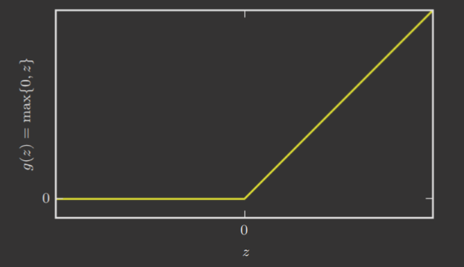
As you may recall, rectified linear units are the default choice. The normal ReLU activation function is

ReLUs are easy to optimize because they are very similar to linear units. Whenever the unit is active, i.e. $z>0$, the gradients remain large and consistent (derivative is $1$) and the second derivative is $0$. Therefore, learning is easier for ReLU compared to other activation functions that introduce second-order effects.

With ReLU being applied to an affine transformation, i.e.

it's also typical to initialize the elements of $\boldsymbol{b}$ to a small positive value to ensure that each ReLU is initially active for most inputs (and thus ensure nonzero gradients at the beginning of training).

As one might imagine, one major drawback of ReLUs is their inability to learn when inactive, i.e. $z<0$. Thus, many ReLU generalizations attempt to address this issue, and are represented by the following function when $z_{i}<0$.

where $\alpha_{i}\neq0$.

Absolute value rectification fixes $\alpha_{i}=-1$ to obtain $g(z)=\lvert z \rvert$. Leaky ReLU fixes $\alpha_{i}$ to a small value, e.g. $0.01$. Parametric ReLU or PReLU treats $\alpha_{i}$ as learnable.

Maxout units are a different generalization that is not element-wise application. They separate $\boldsymbol{z}$ into groups of $k$ values, and each maxout unit outputs the maximum element of its group. Formally,

where $\mathbb{G}^{(i)}$ corresponds to (the indices of) the elements of group $i$. This essentially represents learning a piecewise linear, convex function with $k$ pieces.

In essence, maxout units are essentially learning the activation function itself—with large enough $k$, a maxout unit can approximate any convex function.

Maxout units may also be able to reduce the size of the next layer. They're additionally provided redundancy that resists catastrophic forgetting, where neural networks forget tasks they were previously trained on.

In general, the ReLU and its generalizations are inspired by the principle that models are easier to optimize with linear-like behavior.

Logistic Sigmoid and Hyperbolic Tangent

Prior to the ReLU, most neural networks used either the logistic sigmoid activation function

or the hyperbolic tangent activation function

However, their use in hidden units is now discouraged. This is primarily because these units saturate across most of their domain, translating to vanishing gradients during learning. Their continued use as output units is applicable to gradient-based learning because the appropriate cost function can counteract the saturation.

If a sigmoidal unit is desired or necessary, however, the hyperbolic tangent frequently performs better, as it resembles the identity function more closely since $\tanh(0)=0$ while $\sigma(0)=\frac{1}{2}$. Thus, training a neural network like $\hat{y}=\boldsymbol{w}^{\top}\tanh(\boldsymbol{U}^{\top}\tanh(\boldsymbol{V}^{\top}\boldsymbol{x}))$ resembles training a linear model $\hat{y}=\boldsymbol{w}^{\top}\boldsymbol{U}^{\top}\boldsymbol{V}^{\top}\boldsymbol{x}$ when activations are kept small.

Sigmoidal-like activation functions, despite their disuse in feedforward networks, are seen in other settings, such as recurrent networks.

Other Hidden Units

It's possible to have $g$ be simply the identity function (i.e. equivalent to no activation function). However, this results in some layers becoming entirely linear—this is generally only used to reduce the number of model parameters.

The softmax function may also be used as a sort of "switch"; this is typically applicable to architectures that specifically manipulate memory, which we discuss further in Chapter 10.

Some other common hidden types are

• Radial basis function: saturates to $0$ for most $x$.
• Softplus: smooth ReLU, empirically ReLU is better
• Hard $\tanh$: $g(a)=\\max\{ -1,\min\{ 1,a \} \}$.

6.4 Architecture Design

Architecture denotes the overall network structure. The main considerations for chain-based architectures is network depth and the width of each layer.

Universal Approximation Properties and Depth

The universal approximation theorem states that "a feedforward network with a linear output layer and at least one hidden layer with any 'squashing' activation function (such as the logistic sigmoid activation function) can approximate any Borel measurable function from one finite-dimensional space to another with any desired non-zero amount of error, provided that the network is given enough hidden units." A Borel measurable function, for our purposes, describes a continuous function on a closed and bounded subset of $\mathbb{R}^{n}$.

However, there is no guarantee that the learning algorithm will choose the correct parameters. Moreover, a single layer network may require an exponentially large width for the hidden layer.

Thus, it's useful to extend the number of hidden layers to reduce the number of units necessary to learn the desired function. In fact, many families of functions can only be efficiently (non-exponentially) approximated with a depth $>d$, for some $d$.

An intuitive, geometric explanation for this exponential advantage of deeper networks arises from absolute value rectification, in which each additional hidden layer essentially "folds" the input space, allowing the representation of essentially $2^{l}$ linear regions/pieces of a piecewise function, where $l$ is the depth.

More precisely, the number of linear regions represented by a deep rectifier network with $d$ inputs, depth $l$, and $n$ units per hidden layer is

Generally speaking, though, extending the depth of a model is frequently a useful prior.

Other Architectural Considerations

There are many special architectural designs for specific tasks. We leave such details for later, when we discuss such architectures.

6.5 Back-Propagation and Other Differentiation Algorithms

The evaluation of an input $\boldsymbol{x}$ by a feedforward network to produce an output $\hat{\boldsymbol{y}}$ is known as forward propagation. During training, this produces a scalar cost $J(\boldsymbol{\theta})$. The back-propagation or backprop algorithm propagates this value backwards through the network, computing the gradient used for the actual descent algorithm.

Formally, backprop computes the gradient $\nabla_{\boldsymbol{x}}f(\boldsymbol{x},\boldsymbol{y})$ for some function $f$, where $\boldsymbol{x}$ is a set of variables whose derivatives are desired and $\boldsymbol{y}$ is an additional set of variables whose derivatives are not desired. For machine learning, this is typically $\nabla_{\boldsymbol{\theta}}J(\boldsymbol{\theta})$.

Computational Graphs

Computational graphs help us more formally visualize the structure of operations like back-propagation.

• Each node in the graph corresponds to a variable.
• An operation is a simple function of one or more variables that returns a single output variable.
• If $y$ is computed by applying an operation to a variable $x$, a directed edge is drawn from $x\to y$.

Chain Rule of Calculus

We briefly review chain rule.

For scalars, with $y=g(x)$ and $z=f(y)$,

For vectors, with $\boldsymbol{x}\in \mathbb{R}^{m},\boldsymbol{y}\in \mathbb{R}^{n}$, $g:\mathbb{R}^{m}\to \mathbb{R}^{n}$, $f:\mathbb{R}^{n}\to \mathbb{R}$, $\boldsymbol{y}=g(\boldsymbol{x})$ and $z=f(\boldsymbol{y})$,

For tensors, where the variables and functions are defined analogously,

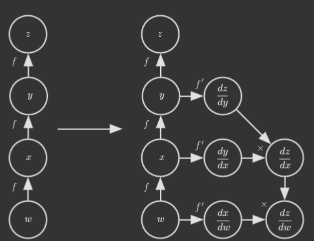
Recursive Chain Rule $\to$ Backprop

I won't go into the mathematics behind this. But, I think it should be pretty intuitive how this works.

The more critical realization here is the use of memoization to store computed derivatives across propagation; otherwise, the algorithm would experience an exponential explosion.

Symbol-to-Symbol Derivatives

Algebraic expressions and computational graphs operate on symbols, and are thus known as symbolic representations. This motivates two different approaches to backprop:

• Symbol-to-number: given a computational graph and the numerical values of the inputs, return a set of numerical values describing the gradients. (Used by PyTorch)
• Symbol-to-symbol: given a computational graph, add additional nodes that provide a symbolic description of the desired derivatives, and then run computations on the graph later given the numerical values of he inputs. (Used by TensorFlow). This approach has the advantage of being able to differentiate the derivatives and produce higher derivatives. A diagram of an example transformation is shown below.

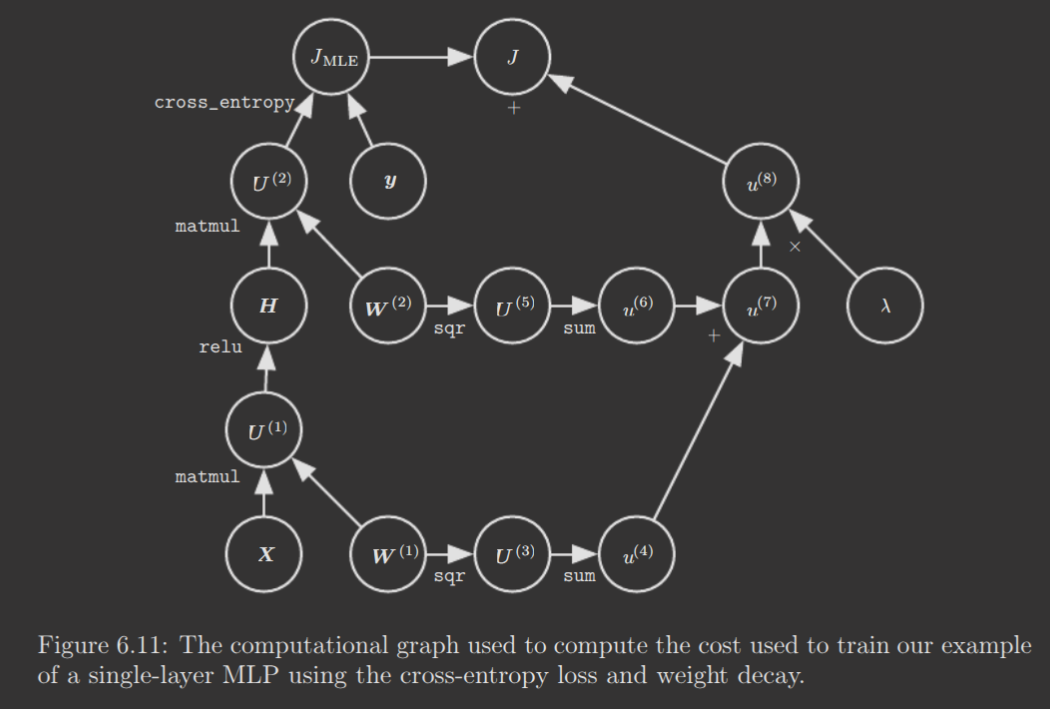
MLP Back-Propagation

I think MLP backprop can be sufficiently understood via a single diagram displaying backprop of a single layer network. No need to understand it in detail; just note the computational graph displays precisely the operations of the MLP and the gradient is computed on this graph starting from the loss function $J$ and proceeding backward, in a postorder DFS manner. (Think reverse topological sort, since the computational graph is a DAG).

Complications

There are some real-world issues that increase the complexity of actual backprop implementations. We won't discuss them in detail; just know they do exist!

Differentiation outside Deep Learning

The field of automatic differentiation discusses, well, automatic, algorithmic computation of derivatives. Backpropagation is a member of a broader class of techniques in this field known as reverse mode accumulation—as one might imagine, this describes the backwards, propagative calculation of derivatives through a computational graph such as the one produced by an MLP. In general, though, determining the optimal sequence of operations to compute the gradient is an $\mathrm{NP}$-Complete problem. There do, however, exist some optimizations implemented in modern deep learning software.

Forward mode accumulation is also potentially preferable when the number of outputs of the graph is larger than the number of inputs; it is to reverse mode as matrix left-multiplication is to matrix right-multiplication. Typically, though, machine learning deals with problems with many input features and few output features. This has seen some consideration for recurrent networks, though (which frequently have many output features).

Higher Order Derivatives

As aforementioned, some symbol-to-symbol software libraries can compute higher order derivatives. However, this has some issues. For second derivatives, for instance, we're interested in the properties of the Hessian matrix. For a function $f:\mathbb{R}^{n}\to \mathbb{R}$, though, the Hessian matrix is of dimensions $n\times n$—when $n$ is in the billions, this quickly becomes intractable.

Instead, deep learning typically leverage Krylov methods, a set of iterative techniques that approximate the properties of the Hessian without explicitly computing it.