Chapter 5: Machine Learning Basics
5.1 Learning Algorithms
"A computer program is said to learn from experience with respect to some class of tasks and performance measure , if its performance at tasks in , as measured by , improves with experience ."
The Task,
ML tasks are typically described in terms of an example, a sample collection of quantitative features of an actual object/event. It is typically represented as a vector of features. Some common tasks include
- Classification: produce .
- Classification w/ missing inputs.
- Regression: produce .
- Transcription: images words.
- Machine translation: languages.
- Structured output: output is a vector with relationships between elements, e.g. sentence
- Anomaly detection: unusual behavior/data
- Synthesis and sampling: create novel output, variation desired
- Data imputation: fill in missing values
- Denoising: clean corrupt example, i.e. predict .
- Density estimation or probability mass function estimation: learn .
The Performance Measure,
For classification and similar tasks, accuracy is measured. The error rate is what's actually used, and is called the expected - loss, where refers to a correct classification and refers to an incorrect classification.
For density estimation and similar tasks, metrics like the average log-probability are used.
Additionally, the model is typically trained on a subset of the dataset known as the training data, while testing is performed on the rest of the dataset, known as testing data. This allows evaluating if the model generalizes to real world data.
The Experience,
ML algorithms are broadly categorized as unsupervised (learn properties/structure of unlabeled dataset, i.e. learn ) or supervised (associate labels with data patterns in labeled dataset, i.e. learn ).
Notably, the chain rule of probability shows that an unsupervised learning problem can be solved by splitting it into supervised learning problems. Similarly, a supervised learning problem can be solved by solving several related unsupervised learning problems. Thus, they are not entirely separate concepts; however, they do roughly categorize the algorithms we consider.
Other learning algorithms include:
- Semi-supervised learning: dataset with labeled and unlabeled data
- Multi-instance learning
- Reinforcement learning: feedback loop with environment
A dataset can frequently be described with a design matrix, which just consists of a different example in each row. This does, though, require each data point to have the same features. Alternatively, for heterogeneous data points, they may be described as a set containing vectors of possibly different sizes. Supervised learning is additionally provided a vector of labels for each data point.
Example: Linear Regression
Linear regression attempts to build a linear (or, really, affine) function . Let be the model's prediction. In the linear-only model,
where is a vector of parameters which essentially act as weights for the features.
For the performance matrix, one possible measure is the mean squared error of the model on the test set .
Or
Training the model involves minimizing , which requires solving for when the gradient is .
Which eventually leads to
Where is the design matrix of the training data.
Note that the system of equations that leads to this solution is known as the normal equations.
5.2 Capacity, Overfitting and Underfitting
The central challenge of ML is the generalization of a model to unseen input.
This is the motivation behind separating the dataset into a training set and test set, and running the algorithm to minimize training error while evaluating on the test set to observe the test or generalization error, which we also want to minimize (though not directly).
So, how exactly can we relate the two to ensure that minimizing the training error also minimizes the test error? We can turn to some ideas from statistical learning theory.
First, we typically make some assumptions about the data generation—in particular, that the individual data points are sampled i.i.d, independently and identically distributed, from the same probability distribution, known as the data generating distribution .
This immediately ensures that for any randomly selected model (not trained, just any arbitrary model). This is simply because the data sampling process was the same for both datasets.
For a trained model, however, this is different since we explicitly minimize the training error. Thus, for a trained model, . A model's effectiveness is determined by its ability to
- Minimize the training error
- Minimize the gap between the training and test error
These two factors correspond precisely to two important challenges in ML: underfitting and overfitting. Underfitting describes when the model is not able to sufficiently minimize training error. Overfitting describes when the gap between the training and test error is excessive.
We can control this, though, by changing a model's capacity—a measure of how many functions a model can fit. Low capacity models tend to underfit as it has a limited selection of functions, while high capacity models tend to overfit as it may select a function too specific to the training dataset.
The most intuitive way to control a model's capacity is to control its hypothesis space, the functions that the learning algorithm is allowed to select as a solution. For instance, the linear regression algorithm allows us to choose any affine function. However, we can also produce quadratic, cubic, quartic, or even higher degree functions to expand the model's hypothesis space, and consequently its capacity as well.
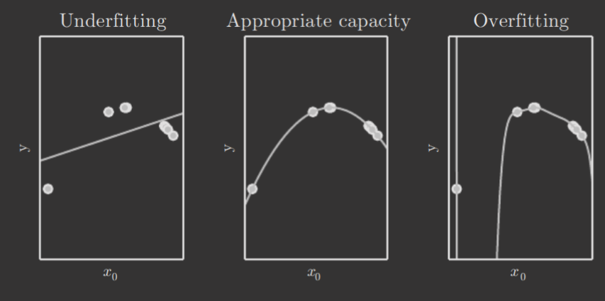
Selecting a model's hypothesis space is, in general, not an easy task and often specific to the problem itself and its complexity. For example, here's the fitting of a quadratic dataset by a linear, quadratic, and degree polynomial, respectively.
Notably, there are some additional terms for capacity. Representational capacity refers to the family of functions a learning algorithm can choose from when varying parameters. However, finding the best function in this family is generally a very difficult optimization problem; thus, the algorithm's effective capacity may be less than the model's representational capacity.
There are also ways to quantify capacity, such as the Vapnik-Chervonenkis dimension (VC dimension), which measures the capacity of a binary classifier (i.e. high VC dimension means high capacity). It is the largest possible value of that a model can "shatter," i.e. for which there exists a training set of different points that the classifier can correctly label. Such quantifiers allow upper-bounding a mode's generalization error; however, they are typically too loose to use in practice for deep learning.
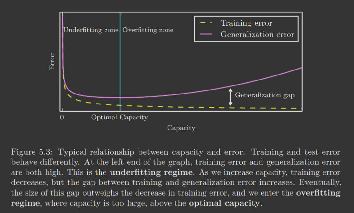
Note the following graph of underfitting/overfitting vs. capacity.
So, how high can capacity be? We can reach arbitrarily high levels via non-parametric models. So far, we have only observed parametric models, which learn a function described by a finite, fixed-size parameter vector. In contrast, non-parametric functions can change the size of their parameter vector while observing data, i.e. update the size while training.
One simple non-parametric algorithm is nearest neighbor regression. This algorithm simply stores the entire training set, and when asked to classify an example, simply returns the value of the nearest "neighbor" in the training set. Mathematically, where (or some other norm, even a learned distance metric!).
One could also simply wrap a parametric learning algorithm inside another that changes the number of parameters as needed.
So, how good can these models become? Well, the ideal model is an oracle that knows the true data generating probability distribution itself. However, due to noise in the distribution, it will still incur some error—this error is known as Bayes error. No model can do better than Bayes error, clearly. Non-parametric models asymptote to Bayes error provided more and more data, while fixed parametric models with suboptimal capacity asymptote to an error value higher than Bayes error. (This applies only to test error; training error can become arbitrarily low).
The No Free Lunch Theorem
The No Free Lunch Theorem states that, averaged over all possible data generating distributions, every classification algorithm has the same error rate when classifying previously unobserved points. That is, no ML algorithm should perform universally better than every other algorithm on every arbitrary dataset. Of course, for real world applications, we only really care about the probability distributions we encounter in the real-world, which we can design algorithms for since we're not seeking some universal learning algorithm.
Regularization
Regularization is essentially the process of incentivizing an algorithm to prefer one type of solution over another.
One type of regularization is weight decay, which motivates the algorithm to choose a set of weights that has a smaller norm. In particular, we describe the objective to minimize as .
where is chosen before training; higher values of encode a stronger preference for small weights. Like capacity tuning, this requires careful selection. Large could underfit, and small could overfit.
The choice of is actually derived from the generalized Lagrangian we discussed in section 4.4. After placing a constraint of for some threshold , is derived and then included in the cost function being minimized, as shown in the generalized Lagrangian. Generally speaking, . (Source).
More generally, we can apply a penalty known as a regularizer to the cost function. In this case, . This is more general than simply including/excluding functions from a hypothesis space, as an exclusion of a function represents an infinitely strong preference against it. Regularizers apply a sliding scale of preference.
Formally, regularization is any modification to a learning algorithm intended to reduce its generalization/test error but not its training error.
We discuss regularization in much greater detail in Chapter 7.
5.3 Hyperparameters and Validation Sets
ML algorithms typically have several tunable settings—think capacity, learning rate, etc. These are known as hyperparameters.
A setting is typically chosen because the hyperparameter is difficult for the learning algorithm to optimize itself or, more usually, it doesn't make sense to learn the hyperparameter on the training set. For instance, if capacity was learned, the model would always choose the maximum capacity to minimize training error as best as possible, resulting in overfitting.
Therefore, it's often necessary to use a validation set of data points. The test set can't be used, so the training data is typically split into a training set, for learning model parameters, and a validation set, for tweaking hyperparameters by providing a rough estimate of generalization error. An 80/20 training/validation split is common.
Repeated use of the same test set actually results in optimistic evaluations of the generalization error, as models are optimized for the test set error. Thus, the introduction of new, different benchmarks is important for keeping the generalization error measurement true to the real world!
Cross-Validation
Sometimes, a dataset is too small to easily split into a fixed training and test set, as this would lead to statistical uncertainty about the estimated test error. One solution to this is -fold cross-validation. In this procedure, a dataset is split into disjoint subsets. Then, for trials, the th subset of the data is used as the test set and the rest of the data is used for training. This, of course, increases computational cost by a factor of ; however, it results in decent approximations of test error.
5.4 Estimators, Bias, and Variance
Point Estimation
Point estimation attempts to provide the single best prediction of some quantity of interest. In essence, when making a prediction, we simply choose the best option or option associated with the highest probability, as opposed to choosing by randomly sampling from the probabiltiy distribution of the options.
Notation-wise, a point estimate of a parameter is denoted by .
Formally, let be a set of i.i.d. data points. A point estimator or statistic is any function of the data
Of course, a good estimator minimizes the distance from .
We will now approach point estimation from the frequentist perspective. Frequentist statistics, in short, treats probabilities as equivalent to frequencies over a large dataset. The opposing perspective is Bayesian, which we will discuss in further detail soon. For now, for our purposes, the frequentist perspective means we treat the true , as a fixed, but unknown value. Meanwhile, the point estimate is just treated as a function of the data. The most critical distinction, however, is that we treat the data as a random process/sampled from a probability distribution. (And as the parameter underlying this distribution). Therefore, is considered a random variable.
Frequently, we are interested in approximating some function , i.e. predict given . We may assume that , where represents the part of the that is not predictable from (e.g. noise). In function estimation, we attempt to approximate with a model or estimate . In reality, is really just a point estimator in the function space! For example, one may note that linear regression is a constrained version of function estimation.
Bias
An estimator's bias is described by
Recall, of course, that is treated as a random variable, hence we may take its expectation.
An estimator is said to be unbiased if , i.e. . Or, an estimator is said to be asymptotically unbiased if , i.e. .
Example: Bernoulli Distribution
Consider a set of examples sampled i.i.d. from a Bernoulli distribution with mean . (Recall that ).
A simple estimator for this distribution is the mean of the training examples.
Whose expectation we can calculate as
Thus, the estimator is unbiased.
Example: Gaussian Distribution Estimators
Consider a set of examples sampled i.i.d. from a Gaussian distribution , where . Recall
A common estimator of is the sample mean
Again, we can calculate its expectation
Thus, the sample mean is an unbiased estimator of the Gaussian mean parameter.
A common estimator of is the sample variance
Again, compute expectation.
Sorry for how... intimidating the above proof looks like. There's no need to concern yourself too much with the details of the derivation, but here's an explanation of all the nontrivial steps for completeness and your curiosity.
- .
- .
- is sampled from the Gaussian distribution, and thus has variance .
- Substituting .
- .
- , but applied over a large sum.
- and are i.i.d, which includes independence covariance is .
- Result of and substituted into .
- Substituting .
- Linearity of Covariance.
- Same reason as .
- .
- Same reason as .
- Linearity of Expectation.
- Same reason as for , and was just computed before.
- Final step, combining everything together and simplifying.
Also, note that there is a nicer derivation that relies on a clever algebraic trick!
In conclusion, though, the sample variance is a biased estimator, with a bias of
And consequently, we must apply what is known as Bessel's correction to obtain an unbiased sample variance estimator.
As
You may be wondering—why is this correction needed? The book doesn't discuss this, but the idea is that the sample variance has only degrees of freedom.
The sample variance is calculated using the sample mean, which is the center of the sample data. Before calculating the sample mean, you have independent pieces of information, your data points. However, after calculating the center, one might note that the data points themselves are not all independent with respect to the center! After all, the center is calculated using the data points. In fact, you really have independent pieces of information points now—if you disregard one piece of information, then the center appears independent to the rest. In other words, degrees of freedom.
Alternatively, consider the fact that the sample mean is the variance-minimizing value. If the variance of the sample is calculated with respect to the population mean, it will certainly be greater than or equal to the variance with respect to the sample mean. Therefore, dividing by instead of applies a small correcting factor. And the choice of is motivated by the degrees of freedom.
Variance and Standard Error
It's also often useful to compute the variance or standard error (standard deviation) of an estimator. An ideal estimator should exhibit low variance.
Note that we are computing the variance of the estimator. This is not the same as computing an estimator for the variance of the Gaussian, as we did above.
The standard error of the sample mean estimator is
Unfortunately, neither or can substitute for and provide an unbiased estimator of the standard error. However, they are both used in practice, as the square root of the unbiased estimator of variance is a small underestimate, especially for large .
Also, consider, for instance, the variance of the estimator of a Bernoulli distribution. (Derivation left out).
The variance of this estimator decreases as a function of , the number of data samples; this is common in popular estimators.
Balancing Bias and Variance to Minimize MSE
The bias and variance of an estimator measure two different sources of error. Bias measures the expected deviation from the true value. Variance measures the expected deviation from the expected estimator value. It's desirable to minimize both, of course, but tradeoffs exist.
Cross-validation is often used to balance the two. Another method is choosing to minimize the mean squared error, as it actually is a combination of the two metrics.
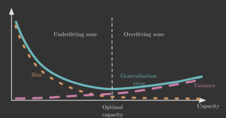
The below diagram shows, for instance, how balancing bias and variance tends to result in minimal generalization error. It also shows the relationship between underfitting/overfitting with bias/variance.
Consistency
Finally, we discuss a desirable property of estimators: consistency, a measure of estimator behavior as the amount of training data, , grows. An estimator is consistent if
where means that, for any , as . This is actually sometimes referred to as weak consistency, with strong consistency meaning almost sure convergence of to , i.e. when for a sequence of random variables converging to .
Consistency implies that bias diminishes as , the dataset size, grows (i.e. asymptotic unbiasedness). Though, one should note that the converse is not true. (e.g. Consider an estimator that bases its estimate off of only the first sample, regardless of ).
5.5 Maximum Likelihood Estimation
The maximum likelihood principle helps guide the derivation of good estimators for different models.
Consider a set of examples independently sampled from the true, but unknown data generating distribution . Let be a parametric family of probability distributions over the same space, where are the parameters (that effectively choose which distribution is used). That is, for some sample , serves as an estimator for this sample's true probability of being sampled from the distribution, .
Then, we define the maximum likelihood estimator (MLE) for as
What does this mean? Well, for each sample from the set of examples , it computes its estimated probability from the model, and then takes the aggregate product. is just the maximizing parameter, i.e. the parameter that maximizes this product.
We formalize the actual reasoning behind the MLE below. But, for intuition, think about a simple example. Let . From the sample, it seems that the true distribution is biased towards . The MLE formula accounts for this, as . Therefore, the MLE will naturally assign a higher estimated probability to , as is implied by the sample dataset.
Due to the imprecision of floating point, and thus the possibility for numerical underflow, MLE is typically computed using logarithms instead.
This doesn't change the arg max because is a monotonically increasing function. Rescaling the cost function also doesn't change the arg max, so this is equivalent to
Where is the empirical distribution defined by the training data.
Now, recall KL divergence from section 3.13.
We can apply this with and .
The first term is a function only of the data generating process, and is thus not affected by the model or the parameter at all. Critically, though, notice how the second term (after applying Linearity of Expectation) is precisely the expression in the arg max of the MLE! Thus, computing , and thus maximizing the expression , is equivalent to minimizing the KL divergence between the empirical distribution (really, the training set) and the model's distribution .
This is also the same as minimizing cross-entropy, which, if you recall from section 3.13, is defined as
In fact, any loss expressed as a negative log-likelihood (NLL) (log-likelihood is ) is really just a measure of the cross-entropy between the empirical distribution defined by the training set and the probability distribution defined by the model. MSE, for instance, is the cross-entropy between the empirical distribution and a Gaussian model.
Thus, we observe that the maximum likelihood estimator is simply matching the model distribution to the empirical distribution as much as possible, which itself is an approximation of the true data generating distribution (which we, of course, cannot access—otherwise the problem's already done :P).
In software, we typically minimize a cost function—thus, in practice, we follow the maximum likelihood principle by minimizing the NLL/cross-entropy.
Conditional Log-Likelihood and MSE
MLE can be generalized to the prediction of a conditional probability . This is important because it's actually what's desired in supervised learning.
Let represent all our inputs and represent all of our observed targets/labels. Then, the conditional MLE is
If the examples are assumed i.i.d., then this is equivalent to
Again, we observe the implicit negative log-likelihood.
MLE: Linear Regression
With this, we can motivate the choice of MSE as the cost function for linear regression.
We consider the model as producing a conditional distribution , and imagine an infinitely large training set, where they may exist several samples with the same input value but different outputs . We define , where predicts the mean of the Gaussian. This is because we expect the different outputs to be normally distributed around the trend's prediction. Since the examples are assumed to be i.i.d., the conditional log likelihood is given by
which simplifies to
Where is the output of the linear regression on the th input . Recall that the MSE is
and we observe that minimizing the MSE is equivalent to maximizing the conditional log likelihood or minimizing the negative conditional log-likelihood, which, as explained previously, produces the maximum likelihood estimator!
Properties of Maximum Likelihood
The primary appeal of MLE is that it is proven to be the best estimator asymptotically, as , in terms of rate of convergence. Under certain conditions, MLE is also consistent. In particular, the conditions are
- The true distribution must lie within the model family .
- The true distribution must correspond to exactly one value of .
There are other consistent estimators. However, they all differ in statistic efficiency—essentially, rate of convergence. It's typically studied in the parametric case, where the MSE of the parameter itself (the estimated vs true parameter) is computed. The Cramer-Rao lower bound shows that no consistent estimator has a lower parameter MSE than the MLE. Thus, maximum likelihood is often the preferred estimator for machine learning.
With smaller datasets, regularization strategies may be applied to increase the bias of MLE but reduce variance.
5.6 Bayesian Statistics
The previous discussions have all been based on frequentist statistics, which make a single estimate of a parameter and make predictions thereafter based on the estimate. The Bayesian approach involves, instead, considering all possible values of when making a prediction. In short, instead of considering the dataset as a random variable sampled from some distribution and the true underlying parameter as some fixed value; Bayesian statistics considers the dataset as fixed, and treats the parameter as a random variable, i.e. treats as if it has an underlying probability distribution.
Bayesian statistics is the more intuitive approach, i.e. you've probably unconsciously used the Bayesian approach in daily life! Recall that frequentist statistics equates probability with long-run frequencies. Bayesian statistics treats probabilities as beliefs, and updates those beliefs as new data becomes available.
Before observing the data, we represent our knowledge of with the prior probability distribution . Generally, the prior is selected to have high entropy to reflect the high degree of uncertainty regarding , such as a Gaussian or uniform distribution.
For some real-world distributions, it might be safe to assume lies in some known range, prior to observing any data.
Many priors are designed to reflect a preference for "simpler" solutions, e.g. smaller parameters.
Now, consider the samples from the dataset. The observation of this data should affect our beliefs about the distribution underlying ; we can compute this via Bayes' rule.
Note that represents the probability of this dataset appearing if our belief about parameterized the probability distribution sampled from. Regardless, the observation of the data induces updates in our posterior probability distribution, i.e. the distribution after observing data, to concentrate around the more likely values of the parameter . This is .
Then, after observing the samples, we can perform predictions on what another (th) sample would be!
In essence, is not just one fixed value; we consider each possible value of with positive probability density, and add its contribution of the probability to the calculation, weighted by the posterior density . Thus, any uncertainty about is considered in every prediction made.
This is in contrast to the frequentist approach, which addresses uncertainty by attempting to minimize variance (and thus minimize uncertainty).
Additionally, unlike the frequentist approach, the Bayesian approach allows the selection of a prior distribution, enabling the expression of preferences like small parameters or smoother models.
However, while Bayesian methods minimize generalization error much better when training data is limited, they incur high computational costs when training data grows large.
Bayesian Linear Regression
I will leave this out for brevity. Refer to the book for a detailed derivation.
Maximum A Posteriori Estimation
Unfortunately, making predictions using the entire Bayesian posterior distribution is generally intractable for large datasets. Therefore, it's common to derive a single point estimate from the Bayesian approach: maximum a posteriori (MAP) is one such method, which simply chooses the with maximal posterior probability density.
On the RHS, the two terms correspond to the usual log-likelihood term and the prior distribution .
As with full Bayesian inference, MAP Bayesian inference may take advantage of the preferences expressed by the prior. For instance, if the prior is , then the log-prior term is proportional to weight decay penalty, and acts the same. This information reduces the variance of the MAP point estimate, relative to MLE, but increases bias.
Actually, some regularized estimation strategies (e.g. weight decay) can often be interpreted as a MAP approximation to Bayesian inference, at least when the regularization involves adding an extra term to the objective function that can correspond proportionally to . This does mean, though, that MAP Bayesian inference provides a more straightforward method of designing complicated regularization terms.
5.7 Supervised Learning Algorithms
Probabilistic Supervised Learning
Most supervised learning algorithms estimate the probability distribution . Maximum likelihood estimation does this for us, finding the best parameter vector for the parametric family of distributions .
We've already seen the application of MLE to linear regression, i.e.
and we can generalize it to the classification scenario by defining a different family of probability distributions.
Let there be two classes, and . As this is a binary classification problem, we only need to define the probability of one class; the other is complementary.
We can transform linear regression into a binary classifier by simply feeding the output of the linear function to the logistic sigmoid function and interpret the output of the logistic sigmoid as a probability (since its range is ).
This is known as logistic regression (but is used for binary classification).
With linear regression, it was possible to directly solve for the optimal weights. With logistic regression, there is no closed-form solution for the optimal parameters; instead, we minimize NLL via gradient descent.
The same strategy—identifying a parametric family of conditional probability distributions with the right input and output—extends to practically any supervised learning problem.
Support Vector Machines
Support vector machines (SVMs) are also based on a linear function . However, in contrast to logistic regression, it outputs only a class, not a probability. An SVM predicts the positive class when , and similarly for the negative class.
The kernel trick is a particularly interesting innovation behind SVMs. It relies on the observation that many ML algorithms can be written exclusively in terms of dot products between examples. The SVM, for instance, can be re-written as
Where is training example and is a vector of coefficients. Note that the expression is essentially measuring the similarity between this training example and the input being evaluated , and dictates how much this should be weighted for the training example .
This small change allows replacing with the output of a given feature function and replacing the dot product with a function known as a kernel.
Note that may not always be the vector inner product/dot product. In infinite dimensional spaces, for example, other kinds of inner products are substituted.
Thus, we have
which is nonlinear with respect to , but linear with respect to and .
So what does this really do? Well, this kernel-based function is equivalent to preprocessing the data by applying to all inputs, and then training a linear model in the new, transformed space. This is important for two reasons.
- It allows learning models nonlinear in using efficient convex optimization techniques, as we consider fixed and optimize only . In particular, may be some nonlinear transformation on the original dataset, i.e. brings a sample in the original input space to a new input space in which the problem solution is linearly representable.
- The kernel function can often be computed more efficiently than the construction and subsequent dot product of two vectors. In essence, for all inputs, but it is implemented differently!
I don't think the book explained the functionality or advantages of the kernel trick particularly well, as a beginner in this field. This Reddit post helped me understand. Wikipedia's explanation is also good.
The most common kernel is the Gaussian kernel.
It's also known as the radial basis function (RBF) kernel, since its "value decreases along lines in space radiating outward from ." Also, note that the RBF corresponds to a dot product in an infinite-dimensional space.
If you're confused by the above, don't worry—just think of the RBF as giving higher weights to closer points. That is, the Gaussian kernel template matches test examples to training examples for prediction. Each training example becomes a template for its label, and, for a test example, the labels of nearby training examples (according to norm) are given higher weights.
You can think of this kernel as taking an input and an example in the training set , and mapping the input into its distance from . In 2D, this can be interpreted as a transformation from the original input space into a polar space with the origin at —at which point is simply equivalent to the radius corresponding to . In dimensions, the interpretation is analogous.
The SVM is not the only algorithm enhanced by the kernel trick, and instead belongs to a larger class of kernel machines or kernel methods.
Kernel machines have some major drawbacks, however.
For instance, the cost of making a prediction is linear in the number of training examples, due to . SVMs are able to mitigate this somewhat by learning a sparse vector, i.e. one with few nonzero elements. Then, classifying a new example only requires evaluating the kernel function for the training examples with nonzero ; these examples are known as the support vectors, and motivate the nomenclature.
Other Simple Supervised Learning Algorithms
We briefly covered nearest neighbor regression previously. -nearest neighbors (kNN) is the family of techniques that extends this algorithm, and is a non-parametric, non-probabilistic supervised learning algorithm. -nearest neighbors, intuitively, doesn't even really learn parameters; instead, during prediction, it simply finds the -nearest neighbors and averages the corresponding values in the training set. For classification, we typically use one-hot encoding, i.e. a vector with and for all other represents the class . The average of the one-hot codes then gives a probability distribution over the classes.
-nearest neighbors can obtain very high accuracy, and it converges to the Bayes error rate as , the training set size, increases. However, it has high computational cost, and generalizes badly with a small training set. Moreover, it cannot distinguish which features are important (i.e. it can't really do what PCA does in identifying the "principal components"). Consider, for instance, a regression task with but only matters for the output. -nearest neighbors will not recognize this, and would require a large dataset to start achieving high accuracy.
A decision tree is another simple supervised learning algorithm. A diagram of one is displayed below.
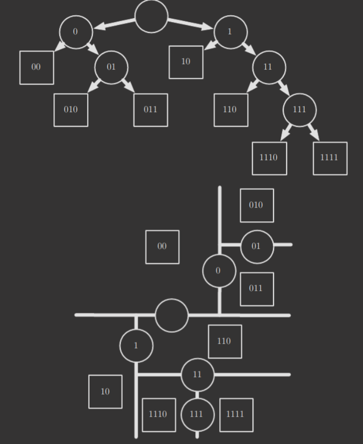
The top half displays the decision tree itself, while the bottom half displays how the decision tree splits the input space. If you're aware of what a K-D tree is, it's similar to that! Essentially, each leaf node corresponds to a category/output, while intermediate nodes correspond to the lines that split the input space. For any test example, it suffices to find the region it corresponds to in the input space by walking the tree, and then returning the output associated with that input space. Decision trees, though, while great for resource-constrained environments for certain types of problems, struggle to solve some problems even easy for logistic regression.
5.8 Unsupervised Learning Algorithms
Principal Component Analysis
PCA, at its core, learns which "axes" of information are more important in the data—allowing it to compress dimensionality by keeping only the most important data.
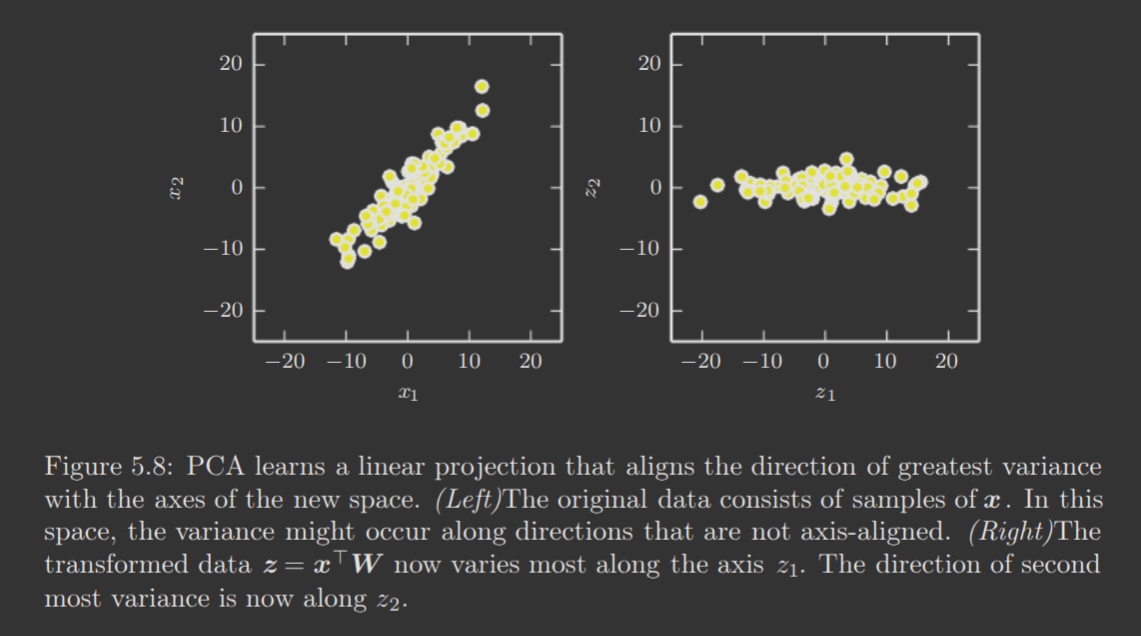
The directions of greatest variance are the principal components, and represent the axes of the new space PCA will transform the data into, in order to compress the data while preserving the most information.
Let some original data representation be , and design matrix. Assume that the data has mean of zero, i.e. . If not, the data can be easily demeaned by subtracting the mean from all examples.
The unbiased sample covariance matrix associated with is described by
PCA effectively performs a linear transformation to a new representation , where is diagonal and is the matrix of the principal components. Note that, typically, , , and , where . This provides the desired dimensionality reduction! The principal components are also the columns of , corresponding to the new axes, as opposed to the dimensions of .
Notably, the principal components of a design matrix are given by the eigenvectors of . (Proof left out). Thus,
Alternatively, they can also be obtained via SVD. In particular, the principal components are the right singular vectors of .
The above simplification results from 's orthogonality implying .
SVD also helps show that PCA provides a diagonal . Noting that means
Again, relying on 's orthogonality for the last step.
The diagonal , meanwhile, implies that the new -representation of the original data via the linear transformation has a diagonal covariance matrix, implying the individual elements of are mutually uncorrelated. In other words, PCA is able to disentangle the unknown factors of variation underlying the data.
-means Clustering
-means clustering partitions the training set into clusters of examples that are near each other (clustering together in the input space). For each input , it provides a -dimensional one-hot code vector such that and all other entries are zero if is in cluster .
The algorithm is simple. First, it initializes different centroids (cluster centers) . Then, it repeats the following two steps until convergence.
- Assign each training example to the nearest centroid 's cluster .
- Update to the mean of all training examples assigned to cluster .
Note that, in general, -means clustering is an NP-Complete problem; however, this algorithm efficiently finds a good approximation for the optimal solution.
5.9 Stochastic Gradient Descent
Stochastic gradient descent (SGD) is an incredibly important deep learning algorithm, and serves as an efficient extension of the classical gradient descent.
Frequently, the cost function of an ML algorithm decomposes as a sum over all the training examples. At each step of gradient descent, the gradient of this cost function must be computed, which has complexity , linear in the number of samples. As the training set grows, this quickly becomes prohibitively slows.
SGD takes advantage of the fact that the gradient is an expectation, and thus may be estimated using only a small subset of samples. For each step, SGD samples a minibatch of examples from the training set where is usually some fixed number much smaller than the training set size. Then, the gradient is estimated as
where is the negative log-likelihood function . (This is just replacing the entire training set with the minibatch). Everything else proceeds equivalently.
SGD has effectively performance has grows, and has phased out the previous popular approach of the kernel trick, which frequently required construction of an matrix (cost of ). We build further on SGD later, in Chapter 8.
5.10 Building an ML Algorithm
Not too much to discuss here.
5.11 Challenges Motivating Deep Learning
Of course, the algorithms described here, while effective, did not generalize to many of the important problems presented in machine learning. Thus, we turn to why these algorithms failed, and why researchers turned to deep learning as a solution.
The Curse of Dimensionality
Frequently, ML problems become exceedingly difficult when the number of dimensions increases. Why? The number of distinct configurations of a set of variables increases exponentially in the number of dimensions.
This poses, for instance, a statistical challenge. The number of distinct configurations may be much larger than the number of training examples—how do we handle configurations for which we have seen no similar example?
Local Constancy and Smoothness Regularization
Recall the purpose of priors—implicit preferences imposed on the learning algorithm. One of the most popular prior is the smoothness or local constancy prior, which states that the learned function should not change much within a small region. Many simpler algorithms rely exclusively on this prior; however, it is insufficient for more sophisticated tasks.
Consider, for instance, -nearest neighbors. In the extreme case, , there are only distinguishable regions. In general, there are only distinguishable regions. Likewise with the decision tree, only distinguishable regions can really be made to achieve some level of statistical confidence in predictions. And, most kernel machines interpolate between nearby training examples, like the -nearest neighbors family, effectively performing what's known as local template matching—suffering from the same problem.
This linearity with the number of training examples is the critical flaw. The space of different configurations is exponential in , but these algorithms' distinguishing regions in the input space are all linear in .
Consider, for instance, extending the checkerboard pattern to dimensions, for some large . Using only the local constancy/smoothness prior and local generalization, we can only really identify points lying in the same checkerboard "square" (hypercube, in -dimensional space) as an existing training example.
Thus, the smoothness assumption and associated non-parametric learning algorithm only work well if there are enough examples for it to observe the most peaks and valleys of the underlying distribution. This is generally true if the distribution is smooth and varies in few enough dimensions.
So how do we represent a more complicated, high-dimensional function, i.e. distinct regions/configurations, with only examples? Well, consider that the checkerboard problem becomes easy if the algorithm is given a prior that implies the periodicity of the checkerboard. In general, the introduction of some additional assumptions about the underlying distribution can help the algorithm.
Of course, strong, task-specific assumptions like the periodicity of the checkerboard are typically not encoded into ML algorithms, so they can generalize well; instead, the core idea of deep learning is that we make the assumption that the underlying data was generated via a composition of factors or features, potentially in some sort of hierarchical fashion. This, and other generic assumptions, actually enable the exponential gain in relationship between the number of examples and the number of distinct regions identifiable by the algorithm. This also helps with the curse of dimensionality.
Manifold Learning
A manifold is a set of points where the local neighborhood around any given point appears to be a Euclidean space. For instance, the Earth is a spherical manifold in 3D space, but is experienced point-wise, by us, as a 2D plane. There is a more formal definition, but this is sufficient for our purposes—take a class on algebraic topology to learn more :)
In machine learning, a manifold tends to mean a connected set of points that can be approximated well considering only a small number of degrees of freedom, or dimensions, embedded in a higher-dimensional space. Think about what PCA does, for instance.
The dimensionality of a manifold may vary between points. A figure eight is a manifold with a single dimension at most points, but two dimensions at the intersection.
Manifold learning algorithms take advantage of this low dimensionality embedded in a high dimensional space by assuming most of the input space is invalid, and that interesting inputs and variations occur only along a collection of small manifolds. This assumption is approximately correct with regards to most AI tasks, and is known as the manifold hypothesis.
First, the probability distribution over real-world items of interest (e.g. images, text, sound) is highly concentrated. Uniform noise never resembles real-world, structured input. This implies the underlying probability distribution is, in reality, highly patterned.
Second, there are frequently many transformations that can be applied to reach similar yet distinct examples in the local neighborhood. A simple example is image transformations, for instance. This motivates the traversal of manifolds, i.e. examples connected to similar examples, and the existence of various small manifolds scattered throughout the input space.
Thus, it's more natural and efficient for machine learning algorithms to learn the low-dimensional manifold underlying the high-dimensional data.