Chapter 4: Numerical Computation

4.1 Overflow and Underflow

Continuous mathematics (i.e. $\mathbb{R}$ ) is not perfectly precise on computers, due to the finite limitations of the real-world. Thus, there can be errors. Underflow is a rounding error that occurs when numbers near zero round to zero, which can significantly impact some functions. Overflow is a rounding error that occurs when numbers with large magnitude are approximated as $\infty$ or $-\infty$ , which often becomes NaN, or Not-a-Number, in software.

Softmax is one such function that is vulnerable to underflow and overflow. It is frequently used to predict probabilities associated with a multinoulli distribution, and is described by

\text{softmax}(\boldsymbol{x}_{i})=\frac{\exp(x_{i})}{\sum_{j=1}^{n} \exp(x_{j})}

Consider an instance in which all $x_{i}=c$ . If $c$ is very negative, $\exp(c)$ will underflow, resulting in a denominator of $0$ . If $c$ is very large and positive, $\exp(c)$ will overflow, resulting in an undefined $\infty$ .

This is commonly resolved by instead evaluating $\text{softmax}(\boldsymbol{z})$ , where $\boldsymbol{z}=\boldsymbol{x}-\mathbf{1}^{\top}\cdot\mathrm{max}_{i}\ x_{i}$ . This ensures the largest argument passed to softmax is $0$ , preventing overflow, and at least one term in the denominator has a value of $1$ (since the $z_{i}$ corresponding to $\arg\max_{i} x_{i}$ is $0$ ).

However, underflow in the numerator can result in the function evaluating to $0$ . This is problematic if we attempt to evaluate $\log\text{softmax}(\boldsymbol{x})$ , which would (erroneously) return $-\infty$ . This can be stabilized in a similar method as above.

4.2 Poor Conditioning

Conditioning describes how rapidly a function changes with respect to changes in the input. A high condition number indicates high sensitivity to changes in input. This is problematic because rounding errors can cause large changes in the output of poorly conditioned functions.

Consider, for instance, the function $f(\boldsymbol{x})=\boldsymbol{A}^{-1}\boldsymbol{x}$ . If $\boldsymbol{A}\in \mathbb{R}^{n\times n}$ has an eigenvalue decomposition, its condition number is

\max _{i,j} \left\lvert \frac{\lambda_{i}}{\lambda_{j}} \right\rvert

Hence, a poorly conditioned matrix would amplify existing errors when multiplying by the inverse.

4.3 Gradient-Based Optimization

Optimization, here, describes the task of minimizing/maximizing some objective function or criterion $f(\boldsymbol{x})$ by iteratively changing $\boldsymbol{x}$ . Typically, minimization is done (as maximization of $f(\boldsymbol{x})$ is the same as minimizing $f(\boldsymbol{x})$ ). For minimization, $f$ may also be called the cost/loss/error function. Also, we frequently denote $\boldsymbol{x}^{*}=\arg\min f(\boldsymbol{x})$ .

Consider a function $y=f(x)$ that we seek to minimize. The derivative $f'(x)$ provides the slope of $f(x)$ at $x$ . Intuitively, this implies that how a small change in the input will impact the output, i.e. $f(x+\epsilon)\approx f(x)+\epsilon f'(x)$ . This is useful, because, in order to reduce $f(x)$ , we can simply move $x$ in small steps in the direction opposite the sign of the derivative. This simple concept is what underlies the famous technique gradient descent (in the 2D case) invented by Cauchy in the 1800s.

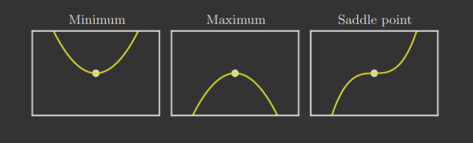
But what if $f'(x)=0$ ? As you may recall, such points are known as critical points or stationary points. These points can be local minimums, local maximums, or saddle points. A 2D representation of all three are provided below.

Of course, local minimum are not necessary the absolute minimum. The absolute minimum of $f(x)$ is known as the global minimum. Optimization is not trivialized by gradient descent because, by nature, gradient descent finds local minimums. For complex, real-world problems filled with many suboptimal local minima, this may not be desirable.

We often consider functions in higher dimensions, too. Note, though, that the function must still have scalar output, i.e. $f:\mathbb{R}^{n}\to \mathbb{R}$ . For functions with higher dimensional inputs, partial derivatives come into play, and the gradient replaces the derivative. The gradient is defined as

\nabla_{x}f(x)=\begin{bmatrix} \frac{ \partial }{ \partial x_{1} } & \dots & \frac{ \partial }{ \partial x_{n} } \end{bmatrix}^{\top}

or the vector of all the partial derivatives of $f$ with respect to its inputs. Meanwhile, critical points are now points where

\nabla _{x}f(x)=\mathbf{0}

The directional derivative in direction $\boldsymbol{u}$ (a unit vector) is the slope of the function $f$ in direction $\boldsymbol{u}$ . In other words, it is

\frac{ \partial }{ \partial \alpha }_{\alpha=0}f(\boldsymbol{x}+\alpha \boldsymbol{u})

By chain rule, this is equivalent to

\boldsymbol{u}^{\top}\nabla_{\boldsymbol{x}}f(\boldsymbol{x})

In order to perform gradient descent and minimize $f$ in higher dimensions, we must compute the direction in which $f$ decreases the fastest. This can be computed using the directional derivative.

\underset{\boldsymbol{u},\boldsymbol{u}^{\top}\boldsymbol{u}=1}{\arg\min}\ \boldsymbol{u}^{\top}\nabla_{\boldsymbol{x}}f(\boldsymbol{x})

This is equivalent to

\underset{\boldsymbol{u},\boldsymbol{u}^{\top}\boldsymbol{u}=1}{\arg\min}\ \lVert \boldsymbol{u} \rVert _{2}\cdot \lVert \nabla_{\boldsymbol{x}}f(\boldsymbol{x}) \rVert \cdot \cos\theta

by the dot product formula. Considering $\lVert \boldsymbol{u} \rVert_{2}=1$ and that $\boldsymbol{u}$ does not influence the value of the gradient, this simplifies to

\underset{\boldsymbol{u}}{\arg\min}\ \cos\theta

Naturally, this is minimized when $\cos\theta=-1\implies\theta=\frac{\pi}{2}$ . In other words, $\boldsymbol{u}$ points in the opposite direction of the gradient. Thus, moving in the direction of the negative gradient produces the steepest descent.

So, this technique suggests a new point

\boldsymbol{x}'=\boldsymbol{x}-\epsilon \nabla_{\boldsymbol{x}}f(\boldsymbol{x})

But what should we set $\epsilon$ to?

$\epsilon$ is known as the learning rate, and essentially determines the step size of the gradient descent. Typically, $\epsilon$ is set to a small value—large step sizes may significantly overshoot the local area in which this negative gradient direction is optimal. An alternative approach is to evaluate $\boldsymbol{x}'$ for several choices of $\epsilon$ , and choose the value that returns the smallest objective function value. This technique is known as line search.

Steepest or gradient descent converges when $\nabla_{\boldsymbol{x}}f(\boldsymbol{x})=\mathbf{0}$ . In most real-world instances, this requires an iterative process; however, it may even be possible to directly compute the critical point by solving the above equation.

info

Gradient descent is specific to continuous spaces. The discrete analogue is known as hill climbing.

Jacobian and Hessian Matrices

Now, we introduce some more advanced mathematical tools for further exploration.

The Jacobian matrix of a function $f:\mathbb{R}^{m}\to \mathbb{R}^{n}$ is a matrix $\boldsymbol{J}(f)\in \mathbb{R}^{n\times m}$ such that $J_{i,j}=\frac{ \partial }{ \partial x_{j} }f(\boldsymbol{x})_{i}$ , i.e. the partial derivative of the $i$ th element of the output of $f$ with respect to the $j$ th element of the input.

The Hessian matrix of a function $f:\mathbb{R}^{n}\to \mathbb{R}$ (scalar output) is a matrix $\boldsymbol{H}(f)(\boldsymbol{x})\in \mathbb{R}^{n\times n}$ such that

\boldsymbol{H}(f)(\boldsymbol{x})_{i,j}= \frac{ \partial^{2} }{ \partial x_{i} \partial x_{j} } f(\boldsymbol{x})

The Hessian can also be interpreted as the Jacobian of the gradient.

Notably, if the second partial derivatives are continuous at some point $\boldsymbol{x}$ , the differential operators are also commutative, i.e.

\frac{ \partial^{2} }{ \partial x_{i} \partial x_{j} } f(\boldsymbol{x})=\frac{ \partial^{2} }{ \partial x_{j}\partial x_{i} } f(\boldsymbol{x})

Thus, $H_{i,j}=H_{j,i}$ , so the Hessian is symmetric at all such points. Since the Hessian is real and symmetric, it has an eigendecomposition!

Consider that the second derivative in a specific direction, represented by unit vector $\boldsymbol{d}$ , can be computed by $\boldsymbol{d}^{\top}\boldsymbol{H}\boldsymbol{d}$ . If $\boldsymbol{d}$ is an eigenvector of $\boldsymbol{H}$ , the second derivative is simply the corresponding eigenvalue. Otherwise, it is a weighted average of the eigenvalues with weights in $(0,1)$ , where eigenvectors whose angle with $\boldsymbol{d}$ is smaller receive higher weights.

Recall from section 2.7 that:

The eigendecomposition of a real symmetric matrix can also optimize quadratic expressions of the form $f(\boldsymbol{x})=\boldsymbol{x}^{\top}\boldsymbol{A}\boldsymbol{x}$ subject to the constraint $\lVert \boldsymbol{x} \rVert_{2}=1$ . The maximum value of $f$ is the maximum eigenvalue, and the minimum is the minimum eigenvalue.

Thus, the maximum eigenvalue of $\boldsymbol{H}$ determines the maximum second derivative, and similarly for the minimum.

It turns out that the directional second derivative can be used as an indicator of how well a gradient step will perform.

2D Second Derivative

You may recall that the second derivative, in two dimensions, describes the curvature of a function, as seen below. What we soon discuss is precisely the same concept, except applied to higher dimensions.

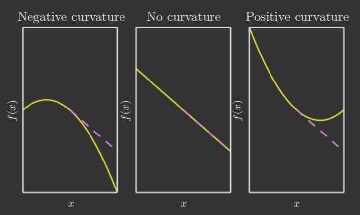
In the content of gradient descent, negative curvature implies the function decreases faster than the gradient predicts. Positive curvature implies it decreases slower, and that large steps can inadvertently increase the cost.

In higher dimensions, we can effectively replace first derivatives with the gradient and second derivatives with the Hessian. So, extending a second-order Taylor series approximation of $f(\boldsymbol{x})$ around the point $\boldsymbol{x}^{(0)}$ to higher dimensions gives

f(\boldsymbol{x})\approx f(\boldsymbol{x}^{(0)})+(\boldsymbol{x}-\boldsymbol{x}^{(0)})^{\top}\boldsymbol{g}+\frac{1}{2}(\boldsymbol{x}-\boldsymbol{x}^{(0)})^{\top}\boldsymbol{H}(\boldsymbol{x}-\boldsymbol{x}^{(0)})

where $\boldsymbol{g}$ is the gradient and $\boldsymbol{H}$ is the Hessian at $\boldsymbol{x}^{(0)}$ . With a learning rate of $\epsilon$ , we find that

f(\boldsymbol{x}')=f(\boldsymbol{x}^{(0)}-\epsilon \boldsymbol{g})\approx f(\boldsymbol{x}^{(0)})-\epsilon \boldsymbol{g}^{\top}\boldsymbol{g}+\frac{1}{2}\epsilon^{2}\boldsymbol{g}^{\top}\boldsymbol{H}\boldsymbol{g}

The three terms in the RHS expression mean, respectively,

The original value of $f$
The expected improvement due to the slope
The correction that should be applied to account for the function's curvature

When the last term $\leq0$ , the Taylor series predicts that $f$ will always decrease as $\epsilon$ increases; in this case, smaller, heuristic choices of $\epsilon$ are used.

Otherwise, when the last term $>0$ , the gradient descent step may move uphill, according to the approximation. Therefore, it suffices to solve for the optimal $\epsilon$ using this equation, which turns out to be

\epsilon^{*}= \frac{\boldsymbol{g}^{\top}\boldsymbol{g}}{\boldsymbol{g}^{\top}\boldsymbol{H}\boldsymbol{g}}

In the worst case, when $\boldsymbol{g}$ aligns with the eigenvector of $\boldsymbol{H}$ corresponding to the maximal eigenvalue $\lambda_{\max}$ , the optimal step size is

\epsilon^{*}= \frac{\boldsymbol{g}^{\top}\boldsymbol{g}}{\lambda_{\max }\boldsymbol{g}^{\top}\boldsymbol{g}}=\frac{1}{\lambda_{\max }}

Therefore, the eigenvalues of the Hessian $\boldsymbol{H}$ determine the scale of the learning rate!

Now, recall the second derivative test in two dimensions. Like how the first derivative test can be extended to higher dimensions with the gradient, so too can the second derivative test with the Hessian.

First, we compute the eigendecomposition of the Hessian matrix at some critical point $\boldsymbol{x}$ . If the matrix...

Is positive definite $\implies$ local minimum,
since the directional second derivative is positive in all directions.
Is negative definite $\implies$ local maximum,
since the directional second derivative is negative in all directions.
Has at least one positive eigenvalue and at least one negative eigenvalue $\implies$ saddle point,
since $\boldsymbol{x}$ is a local maximum on one cross section of $f$ but a local minimum on another.
Otherwise (positive/negative semidefinite), inconclusive.

It may help to refer back to section 2.6 for some of the above definitions.

warning

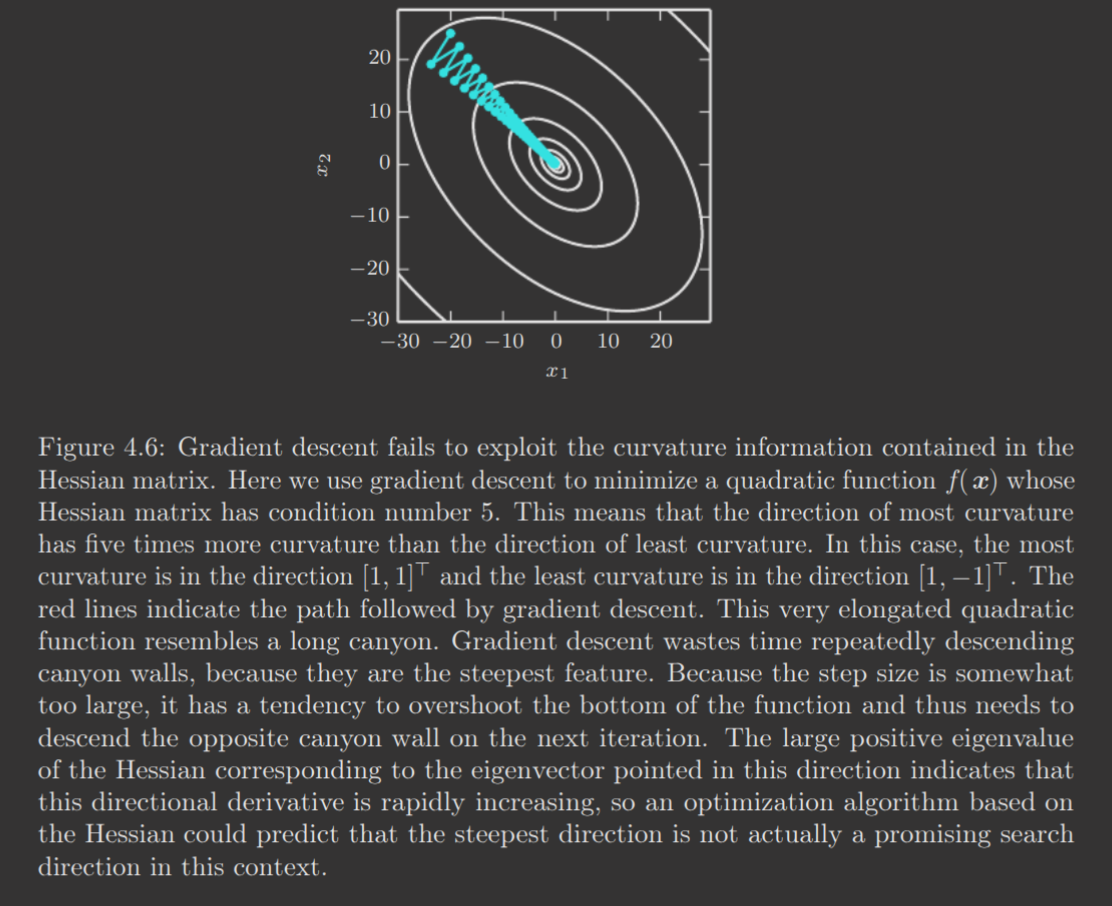
In higher dimensions, the existence of second derivatives in all directions means that the condition number of the Hessian, the measure of how different the second derivatives are from each other, matters. A poor condition number results in gradient descent performing poorly. See below for an example.

This issue can be resolved somewhat via techniques like Newton's method. Newton's method uses the second-order Taylor series expansion (previously shown) to approximate $f(\boldsymbol{x})$ near a point $\boldsymbol{x}^{(0)}$ and then solve directly for the critical point $\boldsymbol{x}^{*}$ of the Taylor series.

\boldsymbol{x}^{*}=\boldsymbol{x}^{(0)}-\boldsymbol{H}\boldsymbol{g}

Where $\boldsymbol{H}$ and $\boldsymbol{g}$ are again the Hessian and gradient evaluated at $\boldsymbol{x}^{(0)}$ .

When $f$ is a positive definite quadratic function, Newton's method applies the above equation once to directly jump to the function minimum. When $f$ can be locally approximated as a positive definite quadratic, Newton's method applies the above equation iteratively.

warning

Newton's method is faster than gradient descent, but fails if nearby a saddle point. It's only appropriate if the nearby critical point is a minimum (the Hessian is positive definite). Gradient descent is more robust in the presence of saddle points.

info

Optimization algorithms that use only the gradient (e.g. gradient descent) are first-order optimization algorithms. Those that also use the Hessian (e.g. Newton's method) are second-order.

Aside: Lipschitz Continuous

The algorithms discussed in this book are applicable to a wide variety of functions; but, as a direct consequence, provide few guarantees. In deep learning, some guarantees can be gained by considering only functions that are either Lipschitz continuous or have Lipschitz continuous derivatives.

A Lipschitz continuous function is a function $f$ whose rate of change is bounded by a Lipschitz constant $\mathcal{L}$ .

\forall \boldsymbol{x},\forall \boldsymbol{y},\ \lvert f(\boldsymbol{x})-f(\boldsymbol{y}) \rvert \leq \mathcal{L}\lVert \boldsymbol{x}-\boldsymbol{y} \rVert _{2}

This property enables quantifying the assumption that a small change in the input will have a small change in the output (by providing an upper bound on the possible change), while remaining a fairly weak constraint applicable to many optimization problems.

Aside: Convex Optimization

Convex optimization algorithms have much stronger restrictions—they apply only to convex functions, for which the Hessian is positive semidefinite everywhere. Such functions lack saddle points, and all of their local minima are global minima. Thus, these algorithms provide many more guarantees; however, many problems in deep learning cannot be solved by convex optimization.

4.4 Constrained Optimization

In some instances, it's desirable to minimize a function $f$ over a subset $\mathbb{S}$ of the possible values of $\boldsymbol{x}$ . This is constrained optimization, and all points $\boldsymbol{x}\in \mathbb{S}$ are known as feasible points.

A simple approach is to simply use gradient descent and then project the result back into $\mathbb{S}$ . Another approach is to design an unconstrained optimization problem whose solution may be transformed into a solution to the original; however, such transformations are difficult to invent and must be designed uniquely for each problem.

The Karsuh-Kuhn-Tucker (KKT) approach is a general solution to constrained optimization. It is, in essence, the generalization of Lagrange multipliers to multiple equality and inequality constraints.

Lagrange Multipliers

Lagrange multipliers is a method to find the minimum (or maximum) value of a function $f:\mathbb{R}^{n}\to \mathbb{R}$ subject to the constraint $g(\boldsymbol{x})=\mathbf{0}$ , for some function $g:\mathbb{R}^{n}\to \mathbb{R}^{m}$ . $g$ is usually interpreted as (or derived from) $m$ constraints. In essence, this solves constrained optimization with only equality constraints.

First, we define a function $\mathcal{L}$ known as the Lagrangian. Note that $\boldsymbol{\lambda}\in \mathbb{R}^{m}$ , and its elements are termed Lagrange multipliers.

L(\boldsymbol{x},\boldsymbol{\lambda}):=f(\boldsymbol{x})+\langle \boldsymbol{\lambda},g(\boldsymbol{x}) \rangle

For our purposes, $\langle .,. \rangle$ can be interpreted as equivalent to the dot product.

L(\boldsymbol{x},\boldsymbol{\lambda}):=f(\boldsymbol{x})+\boldsymbol{\lambda}\cdot g(\boldsymbol{x})

To find the minimum value of $f$ subject to the constraint, we must find all points $\boldsymbol{x}'$ such that they are critical points of the Lagrangian. In other words, all points $\boldsymbol{x}'$ such that

\forall i,\frac{ \partial L }{ \partial x_{i} }_{\boldsymbol{x}=\boldsymbol{x}'} =0 \qquad \forall j,\frac{ \partial L }{ \partial \lambda_{j} }_{\boldsymbol{x}=\boldsymbol{x}'}=0

Computing the partial derivatives returns

\begin{align*} \forall i, \frac{ \partial f }{ \partial x_{i} } +\boldsymbol{\lambda}\cdot \frac{ \partial g }{ \partial x_{i} } &= 0 \\ g(\boldsymbol{x}) &= \mathbf{0} \end{align*}

implicitly evaluated at $\boldsymbol{x}=\boldsymbol{x}'$ .

The first equation provides $n$ equations and the second provides $m$ equations (for each element of $\mathbf{0}$ ). There are $n$ unknowns in the elements of $\boldsymbol{x}'$ and $m$ unknowns in the elements of $\boldsymbol{\lambda}$ . Thus, it suffices to solve the system of linear equations to produce the possible values of $\boldsymbol{x}'$ . Selecting the $\boldsymbol{x}'$ that produces the minimum value for $f(\boldsymbol{x}')$ thus solves the constrained optimization problem.

KKT Conditions

Now, we consider constrained optimization problems consisting of equality and inequality constraints.

Let $f:\mathbb{R}^{k}\to \mathbb{R}$ be the cost function being minimized. Let there be $m$ functions $g^{(i)}:\mathbb{R}^{k}\to \mathbb{R}$ and $n$ functions $h^{(j)}:\mathbb{R}^{k}\to \mathbb{R}$ such that

\mathbb{S}=\{ x\mid \forall i,g^{(i)}(\boldsymbol{x})=0 \land \forall j,h^{(j)}(\boldsymbol{x})\leq 0 \}

The equations involving $g^{(i)}$ are the equality constraints, and those involving $h^{(j)}$ are the inequality constraints.

info

It's also possible to represent the constraints with two vector-to-vector functions $\boldsymbol{g}:\mathbb{R}^{k}\to \mathbb{R}^{m}$ and $\boldsymbol{h}:\mathbb{R}^{k}\to \mathbb{R}^{n}$ , as was done in the Lagrange multipliers section. The reason for the difference in notation is that the Lagrange multipliers section was written while referencing Wikipedia, as the book had no such section.

Next, we introduce the generalized Lagrangian.

L(\boldsymbol{x},\boldsymbol{\lambda},\boldsymbol{\alpha})=f(\boldsymbol{x})+\sum_{i}\lambda_{i}g^{(i)}(\boldsymbol{x})+\sum_{j}\alpha_{j}h^{(j)}(\boldsymbol{x})

Consider that, given $\mathbb{S}\neq \emptyset$ and $f(\boldsymbol{x})\neq \infty$ for any $\boldsymbol{x}$ , then

\min_{x \in \mathbb{S}}f(\boldsymbol{x}) = \min _{\boldsymbol{x}}\max _{\boldsymbol{\lambda}}\max _{\boldsymbol{\alpha},\boldsymbol{\alpha}\geq 0}L(\boldsymbol{x},\boldsymbol{\lambda},\boldsymbol{\alpha})

This is because, any time the constraints are satisfied, we know

\max _{\boldsymbol{\lambda}}\max _{\boldsymbol{\alpha},\boldsymbol{\alpha}\geq 0}L(\boldsymbol{x},\boldsymbol{\lambda},\boldsymbol{\alpha})=f(\boldsymbol{x})

and any time it is violated

\max _{\boldsymbol{\lambda}}\max _{\boldsymbol{\alpha},\boldsymbol{\alpha}\geq 0}L(\boldsymbol{x},\boldsymbol{\lambda},\boldsymbol{\alpha})=\infty

This is because, if $h^{(j)}(\boldsymbol{x}) >0$ for any $j$ , setting $\alpha_{i}=\infty$ results in $L(\boldsymbol{x},\boldsymbol{\lambda},\boldsymbol{\alpha})=\infty$ . Similar reasoning follows with $g^{(i)}$ , though in both directions ( $>0$ and $<0$ ).

Consequently, unconstrained optimization of this expression will always return a feasible point, as all infeasible points are suboptimal.

Unconstrained Optimization of the Lagrangian

In reality, this involves solving a set of $k+m+n$ equations and $2n$ inequalities in $k+m+n$ unknowns. See this blog postfor a more in-depth explanation, though this isn't particularly in scope.

Before we move on, we note some interesting properties of the inequality constraints. Some constraints are tight, i.e. $h^{i}(\boldsymbol{x}^{*})=0$ , while others are not. Such tight constraints are denoted active. This is because the solution $x^{*}$ would remain at least a local solution if an inactive constraint were removed, as it is still a stationary/critical point.

For any inactive constraint, $h^{(i)}(\boldsymbol{x})<0$ . Since $\max_{\boldsymbol{\alpha},\boldsymbol{\alpha}\geq0}$ is included in the expression, $\alpha_{i}=0$ . (Otherwise, the enclosed expression would not be maximized). Intuitively, this is also because this constraint isn't actually affecting the solution locally.

This implies that

\boldsymbol{\alpha}\odot \boldsymbol{h}(\boldsymbol{x})=\mathbf{0}

That symbol $\odot$ means component-wise multiplication—just think $\boldsymbol{\alpha}^{\top}\cdot \boldsymbol{h}(\boldsymbol{x})$ . Thus, this equation means $\alpha_{i}\cdot h^{(i)}(\boldsymbol{x})=0$ , $\forall i$ . In other words, for each constraint, either it is $(1)$ inactive, so that $\alpha_{i}=0$ or $(2)$ active, so that $h^{(i)}(x)=0$ $\implies$ $\alpha_{i}\geq0$ .

(Rant)

The book states "for all $i$ , we know that at least one of the constraints $\alpha_{i}\geq0$ and $h^{(i)}(\boldsymbol{x})\leq0$ must be active at the solution." This took me so long to understand... because they reuse active here to mean whether or not this inequality is true. Why they chose to use "active" to mean this here after defining "active" previously regarding the constraints eludes me.

The KKT conditions provide a simple set of necessary, but not sufficient, conditions for a point $\boldsymbol{x}$ to be optimal.

The gradient of the generalized Lagrangian is $0$ at $\boldsymbol{x}$ .
All constraints on both $\boldsymbol{x}$ and the KKT multipliers (the analogue of Lagrange multipliers for KKT) are satisfied.
The inequality constraints exhibit complementary slackness: $\boldsymbol{\alpha} \odot \boldsymbol{h}(\boldsymbol{x})=\mathbf{0}$ .