Chapter 3: Probability and Information Theory

3.2 Random Variables

A random variable is a variable that can take on different values, each associated with some probability. It may be discrete (finite/countably infinite number of states) or continuous (any real value).

3.3 Probability Distributions

A probability distribution describes the probabilities associated with the values of a random variable. For discrete variables, it is described by a probability mass function (PMF). For continuous variables, the analogue is a probability density function (PDF).

A PMF $P$ must satisfy the following properties

• The domain of $P$ must be the set of all possible states of $\mathrm{x}$
• $\forall x \in \mathrm{x}$, $0\leq P(x)\leq1$.
• $\sum_{x \in \mathrm{x}}P(x)=1$.

A PDF $p$ must satisfy the following, similar properties

• The domain of $p$ must be the set of all possible states of $\mathrm{x}$
• $\forall x \in \mathrm{x},$ $p(x)\geq0$. Notably, it is not required that $p(x)\leq1$.
• $\int p(x) \,\mathrm{d}x=1$.

$p(x)\leq1$ is not required for a PDF because there are an uncountably infinite number of different states of $\mathrm{x}$, and therefore $p(x)>1$ would not cause $\int p(x) \,\mathrm{d}x>1$.

Also, the nomenclature of a PDF (density instead of mass) is motivated by the fact that it does not actually provide the probability of a specific state directly; instead, the probability of landing inside an infinitesimal region with volume $\delta x$ is provided by $p(x)\cdot\delta x$. (After all, the chance of each specific state is effectively $0$, considering the uncountably infinite set of states).

Finally, we note the existence of joint probability distributions, distributions over many variables simultaneously, represented by $P(x_{1},\dots,x_{n})$.

3.4 Marginal Probability

Consider a joint probability distribution. A marginal probability distribution is a probability distribution over a subset of its parameters/variables.

For instance, consider the joint probability distribution $P(\mathrm{x},\mathrm{y})$. Then,

For continuous variables, summation is simply replaced by integration.

3.5 Conditional Probability

Conditional probability is the probability of an event $x$ occurring given the occurrence of another event $y$ has already happened. This is denoted by $P(y\mid x)$, and is calculated as

and is only defined when $P(x)>0$.

3.6 The Chain Rule of Conditional Probabilities

A joint probability distribution over several random variables can be decomposed into the product of several conditional distributions, each over only one variable.

For instance,

The proof of this follows inductively from the definition of conditional probability.

3.7 Independence and Conditional Independence

Two random variables $x$ and $y$ are independent if their probability distribution can be expressed as

Two random variables $x$ and $y$ are conditionally independent given a random variable $z$ if the conditional probability distribution over $v$ and $y$ factorizes in this way (i.e. the above equation) for all values of $z$.

Independence and conditional dependence are denoted $x\perp y$ and $x\perp y\mid z$.

3.8 Expectation, Variance, and Covariance

The expectation or expected value of a function $f(x)$ with respect to probability distribution $P(x)$ is the mean value of $f(x)$ when $x$ is randomly sampled from $P$.

Expectation is linear, i.e. the Linearity of Expectation tells us that

Variance is a measure of how much a function of a random variable $x$ varies across samplings, and is described by

Standard deviation is $\sqrt{ \mathrm{Var}(f(x)) }$.

Covariance describes how closely two values are linearly related.

The covariance of a value with itself is simply the value's variance.

Notably,

Correlation is essentially correlation except each variable is normalized.

The covariance matrix of a random vector $\mathbf{x} \in \mathbb{R}^{n}$ is an $n\times n$ matrix such that $\mathrm{Cov}(\mathbf{x})_{i,j}=\mathrm{Cov}(x_{i},x_{j})$. We note that the diagonal elements of the covariance simply give the variances $\mathrm{Var}(x_{i})$.

3.9 Common Probability Distributions

Bernoulli

A distribution over a single binary random variable, parameterized by a single $\phi \in[0,1]$ such that $P(X=1)=\phi$. It possesses the following properties.

Multinoulli

Also known as the categorical distribution, it describes a single random variable with (finite) $k$ different states—effectively the generalization of a Bernoulli variable. It is parameterized by a vector $\mathbf{p}\in[0,1]^{k-1}$ where $p_{i}$ denotes the probability of the $i$th state and the final, $k$th state's probability is given by $1-\mathbf{1}^{T}\mathbf{p}$. Note that $\mathbf{1}^{T}\mathbf{p}\leq1$ is a necessary constraints.

Gaussian Distribution

Also known as the normal distribution, it is parameterized by $\mu \in \mathbb{R}$, the mean, and $\sigma \in (0,\infty)$, the standard deviation. Its probability density function (PDF) is described by

Frequently, the distribution is parameterized by $\beta \in(0,\infty)$ instead of $\sigma$ where the two are related by $\beta=\frac{1}{\sigma^{2}}$ to make evaluation of the PDF more efficient. $\beta$ is known as the precision or inverse variance. This does not change the distribution's behavior.

The normal distribution is frequently used as a default choice for two reasons.

1. The central limit theorem states that the sum of many independent random variables is approximately normal.
2. The normal distribution encodes the maximum amount of uncertainty over $\mathbb{R}$.

The normal distribution may also generalize to $\mathbb{R}^{n}$ as the multivariate normal distribution, where $\sigma$ is replaced with a positive definite symmetric matrix $\Sigma$ that provides the covariance matrix of the distribution.

Where $x$ and $\mu$ are now vectors instead of scalars. As before, it is possible to replace $\Sigma$ with a precision matrix $\beta=\Sigma ^{-1}$ for increased efficiency of evaluation.

Frequently, the covariance matrix is fixed to be a diagonal matrix. Sometimes, the covariance matrix is also a scalar multiple of the identity matrix, in which case the distribution is known as an isotropic Gaussian distribution.

Exponential and Laplace Distributions

In deep learning, it's often desirable to have a probability distribution with a sharp point at $x=0$. The exponential distribution provides this! It is parameterized by $\lambda$, and is described by

Where $\mathbf{1}_{x\geq_{0}}$ is an indicator function that assigns probability $0$ for all $x<0$.

A related distribution is the Laplace distribution, which places a sharp peak of probability mass at an arbitrary point $\mu$. It is parameterized by $\mu$ and a variable $\gamma$.

The Dirac Distribution and Empirical Distribution

Occasionally, it is desirable to place all probability mass in a distribution at a single point. This can be done by defining a PDF with the Dirac delta function $\delta(x)$, which is parameterized by the desired point $\mu$.

This is essentially defined such that it is zero-valued everywhere except $\mu$, but integrates to $1$.

The Dirac delta distribution is also commonly used to construct an empirical distribution for continuous variable.

Which essentially evenly distributes probability mass across the $m$ points (of some dataset of size $m$) $x_{1},\dots,x_{m}$ (each with $\frac{1}{m}$ mass). This essentially discretizes the distribution. (For discrete variables, the empirical distribution is trivially represented with a multinoulli distribution).

In the context of deep learning, the empirical distribution may represent the proportion of the dataset each item of training data may represent (given possible imbalances in frequencies of training data).

Mixtures of Distributions

It's also possible to define probability distributions by combining several others together. Sampling from such a mixture distribution involves first randomly choosing a component distribution, according to some multinoulli distribution, and then sampling from this component distribution. Thus, the probability of choosing some $x$ from this mixture distribution is

Where $P(c)$ is the multinoulli distribution over the different component distributions. $c$ is known as the component identity random variable.

The mixture model hides a much more interesting concept, which will be discussed in depth later in section 16.5. A latent variable is a random variable that cannot be observed directly. In this case, the component identity random variable $c$ is a latent variable, and is related to the random variable $x$ through a joint distribution, i.e. $P(x,c)=P(x\mid c)P(c)$.

A common type of mixture model is the Gaussian mixture model, in which the components are distinct Gaussian distributions. The parameters of a Gaussian mixture model, beyond its usual means $\mu$'s and covariances $\Sigma$'s, also includes a prior probability $\alpha_{i}=P(c=i)$ for each component $i$. This is just the parameter $\mathbf{p}$ for the multinoulli distribution across the component distributions. Its nomenclature notes that $\alpha_{i}$ represents the model's beliefs about $c$ before it has observed $x$, the result of sampling the Gaussian mixture. Meanwhile, $P(c\mid x)$ is a posterior probability, as it represents the model's beliefs about $c$ after it has observed $x_{i}$.

What does this even mean, though? Well, in real-world instances, where we don't know the distribution that describes a dataset, it's desirable to iteratively compute a closer and closer approximation of the distribution. This is known as Bayesian inference, and Gaussian mixture models are frequently used for this process because they are universal approximators of densities, i.e. any smooth density function/distribution can be approximated with arbitrarily small, nonzero error by a Gaussian mixture model with enough components.

Thus, during Bayesian inference, the prior probabilities represent the model's beliefs about the distribution of the component Gaussians, and the posterior probabilities represent the model's updated beliefs about the distribution after observing a new data point $x$ sampled from the real-world distribution.

3.10 Useful Properties of Common Functions

Some functions commonly appear when working with probability distributions.

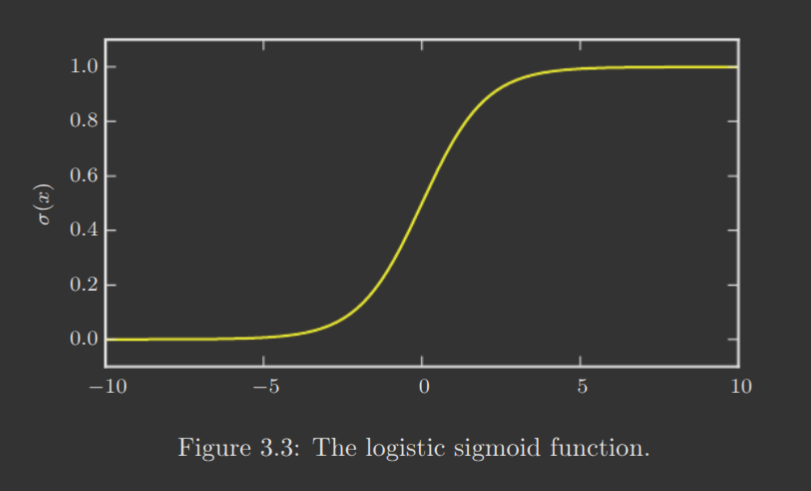
The logistic sigmoid is described by

and is frequently used to produce the $\phi$ parameter of a Bernoulli distribution because its range is $(0,1)$. Notably, the sigmoid function saturates when its argument is very positive or very negative, i.e. $\lvert \frac{\textrm{d}}{\textrm{d} x }\phi \rvert$ becomes small.

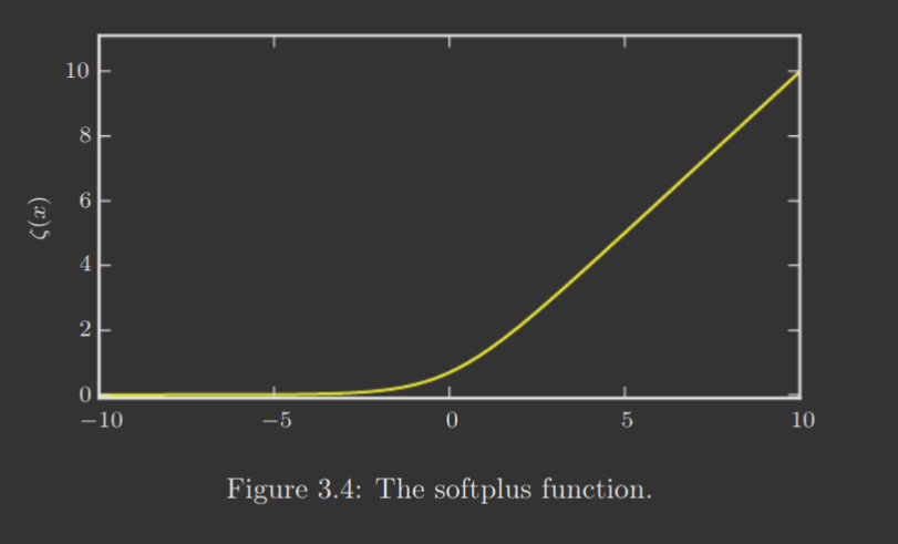
The softplus function is described by

and is frequently used to produce the $\beta$ or $\sigma$ parameter of a normal distribution because its range is $(0,\infty)$. It's also frequently observed when working with sigmoids. Notably, its name describes its initial design—a smoothed or "softened" version of $x^{+}=\mathrm{max}(0,x)$.

Now, a list of some mathematical formulas involving these functions.

Also, note that the last equation, $\zeta(x)-\zeta(-x)=x$, resembles $x^{+}-x^{-}=x$, where $x^{+}=\mathrm{max}(0,x)$ and $x^{-}=\mathrm{max}(0,-x)$. This is partly why $\zeta$ was chosen for "softplus" purpose.

3.11 Bayes' Rule

In essence,

3.12 Technical Details of Continuous Variables

It's necessary to briefly discuss some details of measure theory to formalize some of our notions of continuous variables. For our purposes, we mostly care about measure theory when describing theories that applies to most, but not all, points in $\mathbb{R}^{n}$.

A set of points that is negligibly small is said to have measure zero. Intuitively, this means such a set occupies no volume in the space we are measuring. For instance, in $\mathbb{R}^{3}$, a 3D object has positive measure, but a 2D (polygon) or 1D (line) has measure zero. Also, note that the union of countably many sets that each have measure zero also has measure zero. In particular, the set of all rational numbers $\mathbb{Q}$ has measure zero in $\mathbb{R}$ because $\mathbb{Q}\cong \mathbb{Z}\times \mathbb{Z}$, and $\mathbb{Z}$ has measure zero.

Almost everywhere is also a useful term for us from measure theory. It is a qualifier for a property that holds throughout all of space except on a set of measure zero. As the exceptions occupy a negligible amount of space, they are ignored for most applications. There are some results in probability theory that hold for all discrete values but hold only "almost everywhere" for continuous values.

Finally, another technical detail of continuous variables involves continuous random variables that are functions of one another. Consider random variables $\mathbf{x}$ and $\mathbf{y}$, such that $\mathbf{y}=g(\mathbf{x})$ and $g$ is an invertible, continuous, differentiable transformation. Perhaps contrary to expectations, $p_{y}(\mathbf{y})\neq p_{x}(g^{-1}(\mathbf{y}))$.

Consider, for instance, $g(x)=\frac{x}{2}$ and $\mathbf{x}\sim U(0,1)$, i.e. the uniform distribution over $[0,1]$. If we used the false equation above, i.e. $p_{y}(\mathbf{y})=p_{x}(g^{-1}(\mathbf{y}))$, this would imply $p_{y}(y)=p_{x}(2y)$, which leads to the conclusion $p_{y}(y)=1$ when $y\in\left[ 0, \frac{1}{2} \right]$, and $0$ otherwise. Then, this would imply

which is obviously invalid for a density distribution.

Why is this approach wrong, then? It's because it fails to consider the distortion of space caused by $g$. The probability of $x$ lying in an infinitesimally small region with volume $\delta x$ is given by $p(x)\cdot \partial x$. However, the infinitesimal volume surrounding $x$ in $x$ space may have different volume in $y$ space, since $g$ can transform the scale of space.

We can correct the issue, though. We just need to preserve

We can derive from this

In higher dimensions, $\frac{ \partial g(x) }{ \partial x }$ generalizes to the determinant of the Jacobian matrix, i.e. the matrix with $J_{i,j}=\frac{ \partial x_{i} }{ \partial y_{j} }$.

3.13 Information Theory

Information theory is the study of quantifying how much information is present in a signal. However, it's useful for us to characterize probability distributions or quantify similarity between distributions.

The fundamental idea in information theory is that learning that an unlikely event has occurred is more informative than learning that a likely event has occurred. More specifically,

• Likely events have low information content. Guaranteed events have zero information content.
• Less likely events should have higher information content.
• Independent events should have additive information, e.g. learning a coin came heads up twice conveys twice as much information that learning a coin came heads up once.

A metric that satisfies all three of the above properties is the measure of the self-information of an event $x$.

With $\log=\ln$, $I(x)$ is in the units of nats. One nat is the amount of information gained by observing an event of probability $\frac{1}{e}$. Had we used $\log=\log_{2}$, this would be replaced by bits or shannons. The idea is the same, however.

This function can naturally be applied to discrete variables. However, continuous variables lose some properties—an event with unit density (i.e. a single point in the continuous domain) has zero information, despite not being guaranteed to occur.

Self-information also considers only a single outcome. The uncertainty in an entire probability distribution can be quantified with Shannon entropy.

This is also denoted $H(P)$, and describes the expected amount of information provided by an event drawn from the distribution $P$. It simultaneously provides a lower bound on the number of bits needed, on average, to encode symbols drawn from a distribution $P$. Nearly deterministic distributions have low entropy; near uniform distributions have high entropy. When $x$ is continuous, Shannon entropy is additionally known as differential entropy.

We can also measure the difference between two distributions $P(x)$ and $Q(x)$ over the same random variable $x$ using Kullback-Leibler (KL) divergence.

For discrete variables, it can be interpreted (in information theory terms) as the extra amount of bits/nats required to send a message containing symbols drawn from a probability distribution $P$ when using a code designed to minimize the length of messages drawn from probability distribution $Q$.

KL divergence has several useful properties.

• $D_{KL}\geq0$.
• $D_{KL}=0$ $\iff$ $P=Q$ exactly for discrete variables or "almost everywhere" for continuous variables

A closely related quantity to KL divergence is the cross-entropy $H(P,Q)=H(P)+D_{KL}(P\parallel Q)$.

Minimizing cross-entropy with respect to $Q$ is equivalent to minimizing the KL divergence, since $H(P)$ is entirely dependent on $P$ (recall that $H(P)$ is the Shannon entropy of a distribution $P$).

3.14 Structured Probabilistic Models

Frequently, in machine learning, we frequently encounter probability distributions over a very large number of random variables, but with relatively few interactions between variables. Using a single function to describe the joint probability distribution is, thus, very inefficient. Instead, it's better to factor the distribution into many factors.

Consider three random variables $a,b,c$, such that $a$ influences $b$ and $b$ influences $c$, but $a,c$ are independent given $b$. Then, we can factor the probability distribution as

These factorizations significantly reduce the number of parameters required to describe the distribution, as each distribution $p(\dots)$'s number of parameters is exponential in the number of variables in $(\dots)$. (e.g., $p(a,b,c)$ has $O(3^{n})$ parameters while $p(a)$ has $O(1^{n})$).

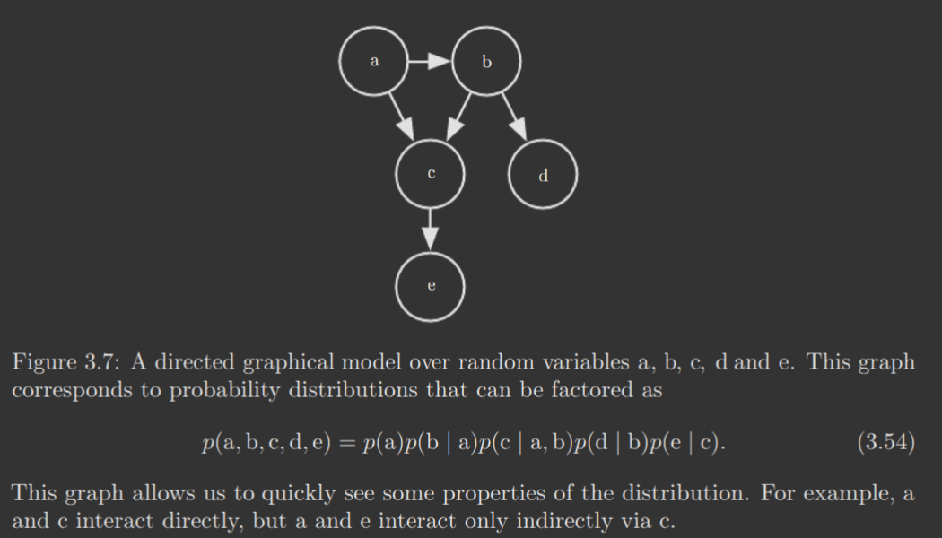
A probability distribution's factorization is frequently described using a graph, known as a structured probabilistic model or graphical model.

There are two types of structured probabilistic models: directed and undirected. In both graphs, each node corresponds to a random variable, and each edge $(u,v)$ denotes a direct interaction between $u$ and $v$.

Directed models represent factorizations into conditional probability distributions, like above. In particular, a directed model contains one factor for every random variable $x_{i}$ in the distribution, and that factor consists of the conditional distribution over $x_{i}$ given the parents of $x_{i}$, denoted $P_{a_{\mathcal{G}}}(x_{i})$.

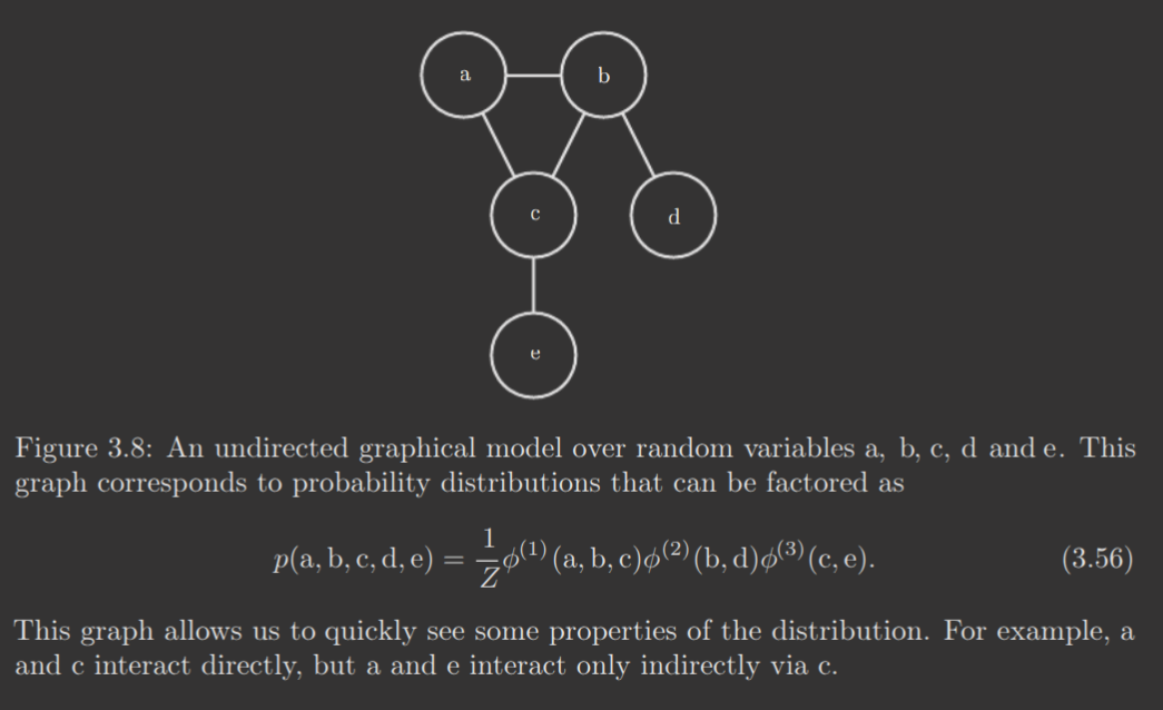
Undirected models represent factorizations into a set of functions that are typically not probability distributions. Any subset of nodes that is fully connected in $\mathcal{G}$ is called a clique. Each clique $\mathcal{C}^{(i)}$ in an undirected model is associated with a factor $\phi^{(i)}(C^{(i)})$, which, again, is not a probability distribution but any function such that its range is nonnegative.

The probability of a certain assignment/results of the random variables is proportional to the product of all of these factors, when provided the input of the assignment. In order to convert this to probabilities, a normalizing constant $Z$ is applied, where $Z$ is the sum or integral of all states of the $\phi$ functions and

Notably, these two graphical representations of factorizations do not denote two mutually exclusive families of probability distributions; a probability distribution may be described with either method.