Chapter 14: Partial Derivatives

14.1 Functions of Several Variables

First several pages of this chapter are just boring explanations of two-variable functions...

Level Curves

The level curves of a function $f$ of two variables are the curves with equations $f(x,y)=k$, where $k$ is a constant (in the range of $f$).

14.2 Limits and Continuity

Limits of Multivariate Functions

For a two-variable function,

The definition extends similarly to higher dimensions.

Formally, ($\epsilon-\delta$),

In other words, the distance between $f(x,y)$ and $L$ can be made infinitesimal by making the distance from $(x,y)$ to $(a,b)$ infinitesimal.

There is one complication with limits for multivariate functions that does not appear in univariate functions, though. Namely, $(a,b)$ can be approached by $(x,y)$ in any direction, infinitely many times. Thus, if there exist more than one direction that $(a,b)$ is approached from and that causes $f(x,y)$ to approach more than one distinct value, the limit of $f(x,y)$ at $(a,b)$ does not exist. Formally,

Continuity

A two-variable function $f$ is continuous at $(a,b)$ if

Also, if $f$ is continuous at every point $(a,b)$ in its domain $D$, then $f$ is continuous on $D$.

Using the properties of limits, it is important to note the following property of continuous functions:

As a result of this fact, all multivariate polynomials, as well as rational functions, are continuous.

Continuity for Proving Limits

If a function is continuous at $(a,b)$, then the limit exists at $(a,b)$. Then, for a function that is a composition of continuous functions, the limit exists at $(a,b)$. This is often helpful for proving that a limit exists at $(a,b)$ for a function! (So you don't have to use an $\epsilon-\delta$ proof).

14.3 Partial Derivatives

Partial Derivatives

A partial derivative of a multivariate function $f$ is essentially just a univariate derivative that considers all other variables constant. Consider a two-variable function $f(x,y)$. Then, the partial derivative with respect to $x$ at $(a,b)$ is denoted $f_{x}(a,b)$ and

Where $g(x)=f(x,b)$.

Similarly, the partial derivative with respect to $y$ is

Where $h(y)=f(a,y)$.

We can also write this in limit definition form.

So, TL;DR, when finding the partial derivative of a multivariate function $f$ with respect to some variable, e.g. $x$, consider all other variables constant when deriving.

With regards to notation, the partial derivative of a multivariate function $f$ with respect to $x$ is

Higher-Order Derivatives

The following are all second partial derivatives of $f$:

Third, fourth, etc. partial derivatives of $f$ are defined similarly.

Most functions we will see will actually have $f_{yx}=f_{xy}$. The following theorem specifies when this occurs:

14.4 Tangent Planes and Linear Approximations

Tangent Planes

Suppose a surface $S$ has equation $z=f(x,y)$, where $f$ has continuous first partial derivatives, and let $P(x_{0},y_{0},z_{0})$ be a point on $S$. Let $C_{1},C_{2}$ be the curves that result from intersecting the surface $S$ with the planes $y=y_{0}$ and $x=x_{0}$. Note that $P$ lies on both $C_{1}$ and $C_{2}$. Le $T_{1}$ and $T_{2}$ be the tangent lines to curves $C_{1}$ and $C_{2}$ at $P$. Then the tangent plane to the surface $S$ at the point $P$ is the plane that contains both tangent lines $T_{1}$ and $T_{2}$.

Note that, for any other curve $C$ that lies on the surface $S$, it passes through $P\iff$ its tangent line at $P$ lies in the tangent plane. In other words, the tangent plane at $P$ consists of all possible tangent lines at $P$, i.e. the tangent plane at $P$ best approximates the surface $S$ near $P$. This will be covered in more detail in 14.6.

Tangent Plane Derivation

A plane passing through $P(x_{0},y_{0},z_{0})$ has the form

Let $a=-\frac{A}{C}$ and $b=-\frac{B}{C}$. Then,

Consider the plane $y=y_{0}$, which intersects with $S$ to form $C_{1}$. Substituting into this equation, we get

Remember that $T_{1}$ is the tangent line to the curve $C_{1}$, and lies in the tangent plane. Therefore, this above equation represents $T_{1}$. We know that the slope of tangent $T_{1}$ can be calculated as $f_{x}(x_{0},y_{0})=\frac{ \partial f }{ \partial x }$. Thus, $a=f_{x}(x_{0},y_{0})$. A similar argument follows for the plane $x=x_{0}$. Hence:

Linear Approximations

Note that the tangent plane equation essentially represents an approximation of the function $f$ at a point $P$ that is a linear function. This function $L$ is called the linearization of $f$ at $P$, and the approximation $f\approx L$ is the linear approximation/tangent plane approximation of $f$ at $P$.

Differentiability

Formally,

In words,

We may also write the following

Differentials

For a univariate function $y=f(x)$, we can write

For a two-variable function $z=f(x,y)$, we can instead write

For a general multivariate function $f(x_{1},x_{2},\dots,x_{n})$,

14.5 Chain Rule

Chain Rule

Recall the chain rule applied to univariate functions $y=f(x)$ and $x=g(t)$:

For multivariate functions, there actually exist several versions of the chain rule. First, we consider the case where $x$ and $y$ are univariate functions.

Now, we consider the case where $x$ and $y$ are multivariate functions.

In other words, just apply the case 1 chain rule separately to $s$ and $t$.

Implicit Differentiation

Suppose that an equation of the form $F(x,y)=0$ defines $y$ implicitly as a differentiable function of $x$, i.e. $y=f(x)$ where $F(x,f(x))=0,\forall x \in \mathrm{Domain}(f)$. If $F$ is differentiable, then we can apply Chain Rule to differentiate $F(x,y)=0$ with respect to $x$:

Now suppose that $z$ is given implicitly as a function $z=f(x,y)$ by an equation of the form $F(x,y,z)=0$, i.e. $F(x,y,f(x,y))=0,\forall(x,y)\in \mathrm{Domain}(f)$. If $F$ and $f$ are differentiable, then we can apply Chain Rule to differentiate the equation $F(x,y,z)=0$ with respect to $x$:

Similarly, by differentiating with respect to $y$, we derive

14.6 Directional Derivatives and the Gradient Vector

Directional Derivative

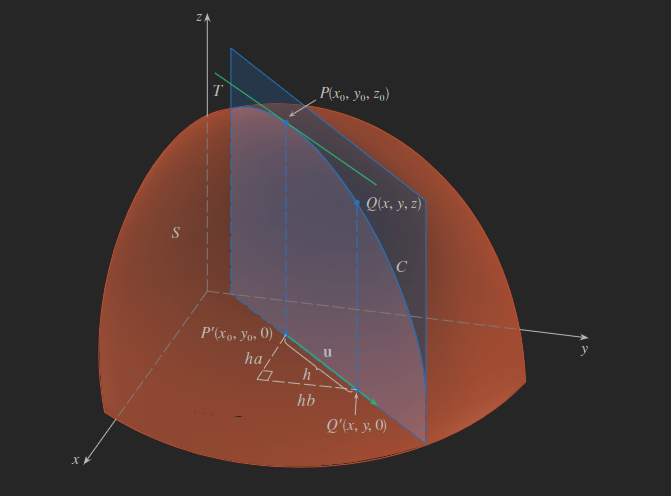
The following diagram may be useful to reference as you read this section:

Consider $z=f(x,y)$. We aim to find the rate of change of $z$ at $(x_{0},y_{0})$ in the direction of the arbitrary unit vector $\mathbf{u}=\langle a,b \rangle$.

Consider the surface described by $z$, and let $z_{0}=f(x_{0},y_{0})$. Then $P(x_{0},y_{0},z_{0})$ lies on $S$. The vertical plane that passes through $P$ in the direction of $\mathbf{u}$ intersects $S$ in a curve $C$. The slope of the tangent line $T$ to $C$ at the point $P$ is the rate of change of $z$ in the direction of $\mathbf{u}$.

Let $Q(x,y,z)$ be another point on $C$. Let $P',Q'$ be the projections of $P,Q$ onto the $xy$-plane. Then, the vector $\overrightarrow{P'Q'} \parallel \mathbf{u}$, and thus

for some scalar $h$. In other words, $x-x_{0}=ha$ and $y-y_{0}=hb$, i.e. $x=x_{0}+ha$ and $y=y_{0}+hb$. Therefore,

Taking the limit as $h\to 0$, we get

We can rewrite this in a more useful form:

The above follows directly from Chain Rule, and its proof is left as an exercise to the reader. (Hint: consider deriving the function $g(h)=f(x_{0}+ha,y_{0}+hb)$).

Also, if $\mathbf{u}$ make an angle $\theta$ with the positive $x$-axis, we can write $\mathbf{u}=\langle \cos\theta,\sin\theta \rangle$. Then, the formula becomes

Gradient Vector

Note that the directional derivative of $f(x,y)$ can actually be written as a dot product:

The first vector in the dot product appears frequently in many contexts, and so is specially denoted as follows:

We may then rewrite the directional derivative equation again.

In other words, the directional derivative in the direction of $\mathbf{u}$ is the scalar projection of the gradient vector onto $\mathbf{u}$. (Recall $\mathrm{comp}_{a}b=\frac{a\cdot b}{\lvert a \rvert}$, and that $\mathbf{u}$ is a unit vector).

Maximizing the Directional Derivative

We aim to find the maximal directional derivative of $f$ at a given point, i.e. the direction in which $f$ changes the fastest at a given point and the corresponding magnitude of rate of change.

Note that

where $\theta$ denotes the angle between $\nabla f$ and $\mathbf{u}$. The maximum value of $\cos\theta$ is $1$, and occurs when $\theta=0$. Therefore, the maximum value of $D_{u}f$ is $\lvert \nabla f \rvert$, and it occurs when $\theta=0\implies$ $\mathbf{u} \parallel \nabla f$, i.e. the two vectors have the same direction. Thus,

Tangent Planes to a Level Surface

Suppose $S$ is a surface with equation $F(x,y,z)=k$, i.e. it is a level surface of a three-variable function $F$. Let $P(x_{0},y_{0},z_{0})$ lie on $S$ and let $C$ be an arbitrary curve that lies on $S$ and passes through $P$. Let $C=\mathbf{r}(t)=\langle x(t),y(t),z(t) \rangle$, and let $t_{0}\in \mathbb{R}$ such that $P=\mathbf{r}(t_{0})$. Consider that

Now, substituting $t=t_{0}$,

In other words,

If $\nabla F(x_{0},y_{0},z_{0})\neq \mathbf{0}$, we can then define the tangent plane to the level surface at $P(x_{0},y_{0},z_{0})$ as the plane that passes through $P$ and has normal vector $\nabla F(x_{0},y_{0},z_{0})$. Thus,

We can also define a line called the normal line to $S$ at $P$ such that it passes through $P$ and is perpendicular to the tangent plane. The direction of this normal line is clearly the same as the gradient vector, and as such is defined as

14.7 Maximum and Minimum Values

A two-variable function $f$ has a local maximum at $(a,b)$ if $f(x,y)\leq f(a,b)$ when $(x,y)$ is near $(a,b)$. A local minimum is defined analogously.

If $f(x,y)\leq f(a,b)$, $\forall(x,y)\in D$, the domain of $f(x,y)$,then $f(a,b)$ is an absolute maximum. An absolute minimum is defined analogously.

There exist the following tests for finding the local extrema of $f(x,y)$, which are analogous to their univariate counterparts.

Meanwhile, we also consider the absolute extrema of $f(x,y)$ over some closed interval. For $\mathbb{R}^{2}$, a bounded set is one that is contained in some disk. Meanwhile, a closed set is one that additionally contains all its boundary points. With these definitions, we then define the Extreme Value Theorem for two-variable functions.

To find the absolute extrema, we perform the following process.

Notice the similarity to the univariate analogue! However, one major difference is that, when determining the extreme values on the boundary of $D$, it is not possible to calculate the values of every point on the boundary of $D$ (since there are infinitely many!). Instead, it suffices to set constraints on $x,y$ such that $(x,y)$ is on the boundary, and determine the extreme values of $f(x,y)$ over these constraints, typically through taking the derivatives of the consequent univariate functions. It may be necessary to split the boundary up into multiple different constraints. See the textbook for some helpful examples!

14.8 Lagrange Multipliers

One Constraint

Lagrange's method is a way of maximizing/minimizing a general function $f(x,y,z)$ when a constraint of the form $g(x,y,z)=k$ is considered.

Consider the function $f(x,y,z)$ subject to the constraint $g(x,y,z)=k$. In other words, $(x,y,z)$ is restricted to lie on the level surface $S$ with equation $g(x,y,z)=k$.

Suppose $f$ has an extreme value at a point $P(x_{0},y_{0},z_{0})$ on the surface $S$ and let $C$ be a curve with vector equation $\mathbf{r}(t)=\langle x(t),y(t),z(t) \rangle$ that lies on $S$ and passes through $P$. If $t_{0}$ is the parameter value corresponding to the point $P$, then $\mathbf{r}(t_{0})=\langle x_{0},y_{0},z_{0} \rangle$. The composite function $h(t)=f(x(t),y(t),z(t))$ represents the values that $f$ takes on the curve $C$. Since $f$ has an extreme value at $(x_{0},y_{0},z_{0})$, which corresponds to $t_{0}$ for $\mathbf{r}(t)$, $h$ has an extreme value at $t_{0}$, i.e. $h'(t_{0})=0$. Since $f$ is differentiable, we can apply Chain Rule as follows:

In other words, the gradient vector $\nabla f(x_{0},y_{0},z_{0})$ is orthogonal to the tangent vector $\mathbf{r}'(t_{0})$ to every such curve $C$. From [[#Tangent Planes to a Level Surface|section 14.6]], we know that the gradient vector of $g$, $\nabla g(x_{0},y_{0},z_{0})$, is also orthogonal to $\mathbf{r}'(t_{0})$ for every curve $C$, since $g(x,y,z)=k$ describes the level surface $S$. In other words, $\nabla f(x_{0},y_{0},z_{0})\parallel \nabla g(x_{0},y_{0},z_{0})$. Further, if $\nabla g(x_{0},y_{0},z_{0}) \neq 0$, then $\exists \lambda$ such that

$\lambda$ is called the Lagrange multiplier.

For a 3-variable function, we can write the vector equation $\nabla f=\lambda \; \nabla g$ in terms of its components to transform the equation in step 1 into

This is a system of four unknowns and four equations, so it is solvable!

Two Constraints

We can also find the extreme values of $f(x,y,z)$ subject to two constraints $g(x,y,z)=k$ and $h(x,y,z)=c$. Then, we can write