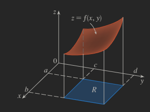
Logo

Chapter 15: Multiple Integrals

15.1 Double Integrals over Rectangles

Derivation

Consider a function ff of two variables bounded by a closed rectangle RR, i.e. bounded by axba\leq x\leq b and cydc\leq y\leq d, for some a,b,c,dRa,b,c,d\in \mathbb{R}. Then, define the 3D solid SS such that it lies between the rectangle RR lying in the xyxy-plane and the surface with equation z=f(x,y)z=f(x,y), bounded by the above bounds. The below image may help you understand this:

double-integrals.png

We aim to find the volume of SS.

Consider dividing rectangle RR into subrectangles, analogous to how we might do a Riemann sum, but instead in 3 dimensions. For any subrectangle, we can approximate the volume of SS lying above the subrectangle by computing f(x0,y0)ΔAf(x_{0},y_{0})\Delta A, where x0,y0x_{0},y_{0} represents an arbitrary point in the subrectangle and ΔA\Delta A represents the area of the subrectangle.

Approximating the volume mathematically, we get

Vi=1mj=1nf(xi,yj)ΔAi,jV\approx \sum_{i=1}^{m} \sum_{j=1}^{n} f(x_{i},y_{j})\Delta A_{i,j}

Where m,nm,n denote the number of subdivisions in each dimension (xx-axis and yy-axis).

To find the true volume, we of course just take the limit:

V=limm,ni=1mj=1nf(xi,yj)ΔAi,jV=\lim_{ m,n \to \infty } \sum_{i=1}^{m} \sum_{j=1}^{n} f(x_{i},y_{j})\Delta A_{i,j}

Double Integral

Mathematically, we often write instead that

Double Integral
V=Rf(x,y)dA=limm,ni=1mj=1nf(xi,yj)ΔAi,jV= \underset{ R }{\iint} f(x,y) \, dA = \lim_{ m,n \to \infty } \sum_{i=1}^{m} \sum_{j=1}^{n} f(x_{i},y_{j})\Delta A_{i,j}

We don't have to use the limit definition to integrate, however. Instead, we can express a double integral, as an iterated integral:

cdabf(x,y)dxdy=cd[abf(x,y)dx]dyabcdf(x,y)  dydx=ab[cdf(x,y)dy]dx\begin{align*} \int_{c}^{d} \int_{a}^{b} f(x,y) \, dx \, dy &= \int_{c}^{d} \left[ \int_{a}^{b} f(x,y) \, dx \right] \, dy \\ \int_{a}^{b} \int_{c}^{d} f(x,y) \,\;\mathrm{d} y \, dx &= \int_{a}^{b} \left[ \int_{c}^{d} f(x,y) \, dy \right] \, dx \end{align*}

Essentially, we can integrate independently of the other integrals. Note also that partial integration works analogously as to partial differentiation, i.e. you treat other variables as constant.

Additionally, note that many functions ff can be integrated in either order when finding the volume of the solid SS.

Fubini's Theorem

If ff is continuous over the rectangle R={(x,y)axb,cyd}R=\{ (x,y) \mid a\leq x\leq b,c\leq y\leq d \}

Rf(x,y)  dA=cdabf(x,y)dxdy=abcdf(x,y)dydx\underset{ R }{ \iint } f(x,y) \,\;\mathrm{d} A = \int_{c}^{d} \int_{a}^{b} f(x,y) \, \mathrm{d}x \, \mathrm{d}y = \int_{a}^{b} \int_{c}^{d} f(x,y) \, \mathrm{d}y \, \mathrm{d}x

Exception: Product of Univariate Functions

In the special case where f(x,y)=g(x)h(y)f(x,y)=g(x)h(y), i.e. can be factored as a product of a function of only xx and a function of only yy, then we can write

Rf(x,y)dA=Rg(x)h(y)dA=abg(x)dxcdh(y)dy\underset{ R }{ \iint } f(x,y) \, \mathrm{d}A =\underset{ R }{ \iint } g(x)h(y) \, \mathrm{d}A = \int_{a}^{b} g(x) \, \mathrm{d}x \int_{c}^{d} h(y) \, \mathrm{d}y

We can do this because yy is constant when integrating with respect to xx, and vice versa.

Average Value

This is calculated analogously to how it is in 1 dimension. Simply,

favg=1A(R)Rf(x,y)dAf_{\mathrm{avg}} = \frac{1}{A(R)}\underset{ R }{ \iint } f(x,y)\,\mathrm{d}A

Where A(R)A(R) is the area of the rectangle RR. This should make sense intuitively.

15.2 Double Integrals over General Regions

We aim to integrate volumes of solids over arbitrary plane regions, not just rectangles. We will consider two types of regions, and their corresponding integrations.

In order to evaluate Df(x,y)dA\iint_{D}f(x,y)\,\mathrm{d}A, we consider a rectangle R=[a,b]×[c,d]R=[a,b]\times[c,d] that contains the plane region DD, i.e. DRD\subseteq R. We define a function FF with domain RR as

F(x,y)={f(x,y)if (x,y) is in D0if (x,y) is in R but not in DF(x,y)=\left\{ \begin{matrix} f(x,y) & \text{if } (x,y) \text{ is in } D \\ 0 & \text{if } (x,y) \text{ is in } R \text{ but not in } D \end{matrix} \right.

Then, if FF is integrable over RR, we have

Df(x,y)dA=RF(x,y)dA\underset{ D }{ \iint } f(x,y)\,\mathrm{d}A = \underset{ R }{ \iint } F(x,y)\,\mathrm{d}A

Type I

A plane region DD is said to be of type I if it lies between the graphs of two continuous functions of xx, that is:

D={(x,y)axb,g1(x)yg2(x)}D=\{ (x,y)\mid a\leq x\leq b,g_{1}(x)\leq y\leq g_{2}(x) \}

Then, we may write

Df(x,y)dA=RF(x,y)dA=abcdF(x,y)dydx\begin{align*} \underset{ D }{ \iint } f(x,y)\,\mathrm{d}A &= \underset{ R }{ \iint } F(x,y)\,\mathrm{d}A = \int_{a}^{b} \int_{c}^{d} F(x,y) \, \mathrm{d}y \, \mathrm{d}x \\ \end{align*}

Note that F(x,y)=0F(x,y)=0 if y<g1(x)y<g_{1}(x) or y>g2(x)y>g_{2}(x). Thus,

cdF(x,y)dy=g1(x)g2(x)F(x,y)dy=g1(x)g2(x)f(x,y)dy\int_{c}^{d} F(x,y) \, \mathrm{d}y = \int_{g_{1}(x)}^{g_{2}(x)} F(x,y) \, \mathrm{d}y = \int_{g_{1}(x)}^{g_{2}(x)} f(x,y) \, \mathrm{d}y

Therefore,

Type I Volume

If ff is continuous on a type I region DD such that D={(x,y)axb,g1(x)yg2(x)}D=\{ (x,y) \mid a\leq x\leq b,g_{1}(x)\leq y\leq g_{2}(x) \}, then

Df(x,y)dA=abg1(x)g2(x)f(x,y)dydx\underset{ D }{ \iint } f(x,y)\,\mathrm{d}A = \int_{a}^{b} \int_{g_{1}(x)}^{g_{2}(x)} f(x,y) \, \mathrm{d}y \, \mathrm{d}x

Type II

A plane region DD is said to be type II if it is between the graphs of two continuous functions of yy, i.e. type I but xx is bounded instead of yy:

D={(x,y)cyy,h1(y)xh2(y)}D=\{ (x,y)\mid c\leq y\leq y,h_{1}(y)\leq x\leq h_{2}(y) \}

Thus, by similar derivation as in [[#Type I]], we find

Type II Volume
Df(x,y)dA=cdh1(y)h2(y)f(x,y)dxdy\underset{ D }{ \iint } f(x,y)\,\mathrm{d}A=\int_{c}^{d} \int_{h_{1}(y)}^{h_{2}(y)} f(x,y) \, \mathrm{d}x \, \mathrm{d}y

Properties of Double Integrals

(1)  D[f(x,y)+g(x,y)]dA=Df(x,y)dA+Dg(x,y)dA(2)  Dcf(x,y)dA=cDf(x,y)dA,  for  some  constant  c(3)  f(x,y)g(x,y),(x,y)D    Df(x,y)dADg(x,y)dA(4)  D=D1D2,D1D2=    Df(x,y)dA=D1f(x,y)dA+D2f(x,y)dA(5)  D1dA=A(D)(6)  mf(x,y)M,(x,y)D    mA(D)Df(x,y)  dAMA(D)\begin{align*} \mathbf{(1)}\;& \underset{ D }{ \iint } [f(x,y)+g(x,y)]\,\mathrm{d}A = \underset{ D }{ \iint }f(x,y)\,\mathrm{d}A + \underset{ D }{ \iint } g(x,y)\,\mathrm{d}A \\ \mathbf{(2)}\;& \underset{ D }{ \iint } cf(x,y)\,\mathrm{d}A = c\underset{ D }{ \iint }f(x,y)\,\mathrm{d}A, \mathrm{\;for\;some\;constant\;}c \\ \mathbf{(3)}\;& f(x,y)\geq g(x,y),\forall(x,y)\in D \implies \underset{ D }{ \iint }f(x,y)\,\mathrm{d}A \geq \underset{ D }{ \iint }g(x,y)\,\mathrm{d}A \\ \mathbf{(4)}\;& D = D_{1}\cup D_{2},D_{1}\cap D_{2}=\emptyset \implies \underset{ D }{ \iint }f(x,y)\,\mathrm{d}A = \underset{ D_{1} }{ \iint }f(x,y)\,\mathrm{d}A+\underset{ D_{2} }{ \iint }f(x,y)\,\mathrm{d}A \\ \mathbf{(5)}\;& \underset{ D }{ \iint }1\,\mathrm{d}A=A(D) \\ \mathbf{(6)}\;& m\leq f(x,y)\leq M,\forall (x,y)\in D\implies mA(D)\leq \underset{ D }{ \iint }f(x,y)\;\mathrm{d}A\leq MA(D) \end{align*}

Where,

15.3 Double Integrals in Polar Coordinates

The proof of the formula for this will be left as an exercise to the reader since it is similar to the proof of double integrals over rectangles. Hint: consider dividing a polar region into polar subrectangles.

Double Integral over Polar Rectangle

If ff is continuous on a polar rectangle RR describe by 0arb0\leq a\leq r\leq b, α0β\alpha\leq {0}\leq\beta, where 0βα2π0\leq\beta-\alpha\leq{2}\pi, then

Rf(x,y)dA=αβabf(rcosθ,rsinθ)rdrdθ\underset{ R }{ \iint } f(x,y) \, \mathrm{d}A = \int_{\alpha}^{\beta} \int_{a}^{b} f(r\cos\theta,r\sin\theta) \cdot r \, \mathrm{d}r \, \mathrm{d}\theta
Note the additional factor of rr on the RHS. Careful not to forget this!

Generalizing to any polar region, similarly to how it was done in 15.2, we get

Double Integral over General Polar Region

If ff is continuous on a polar region of the form

D={(r,θ)αθβ},h1(θ)rh2(θ)D=\{ (r,\theta) \mid\alpha\leq \theta\leq \beta \},h_{1}(\theta)\leq r\leq h_{2}(\theta)

Then

Df(x,y)dA=αβh1(θ)h2(θ)f(rcosθ,rsinθ)rdrdθ\underset{ D }{ \iint }f(x,y)\,\mathrm{d}A = \int_{\alpha}^{\beta} \int_{h_{1}(\theta)}^{h_{2}(\theta)} f(r\cos\theta,r\sin\theta)\cdot r \, \mathrm{d}r \, \mathrm{d}\theta

15.4 Applications of Double Integrals

Density and Mass

Let ρ(x,y)\rho(x,y) denote the density function of a region DD. Thus,

ρ(x,y)=limΔmΔA\rho(x,y)=\lim \frac{\Delta m}{\Delta A}

Where Δm,ΔA\Delta m,\Delta A are the mass and area of an infinitesimal rectangle containing (x,y)(x,y). Thus, it naturally follows that

m=Dρ(x,y)dAm=\underset{ D }{ \iint }\rho(x,y)\,\mathrm{d}A

Physicists consider other types of density that aren't mass as well. For instance, if the charge density if given by σ(x,y)\sigma(x,y) at (x,y)(x,y) in DD, then the total charge QQ is simply

Q=Dσ(x,y)dAQ=\underset{ D }{ \iint }\sigma(x,y)\,\mathrm{d}A

Moments and Centers of Mass

The moment of a particle is the product of its mass and its directed distance from the axis. Consider an infinitesimal rectangle RxyR_{xy} containing the point (x,y)(x,y). Then, the mass of Rxyρ(x,y)ΔAR_{xy}\approx \rho(x,y)\Delta A, and the moment of RxyR_{xy} with respect to the xx-axis is therefore

Mx(Rxy)=ρ(x,y)ΔAyxyM_{x}(R_{xy})=\rho(x,y)\Delta A\cdot y_{xy}

Taking the limit of the sum of these quantities gives us the moment of the entire lamina about the xx-axis:

Mx=Dyρ(x,y)dAM_{x}=\underset{ D }{ \iint }y\rho(x,y)\,\mathrm{d}A

And about the yy-axis,

My=Dxρ(x,y)dAM_{y}=\underset{ D }{ \iint }x\rho(x,y)\,\mathrm{d}A

Using these, we derive the coordinates (x,y)(\overline{x},\overline{y}) of the center of mass of a lamina occupying the region DD:

x=Mym=1mDxρ(x,y)dAy=Mxm=1mDyρ(x,y)dA\overline{x}=\frac{M_{y}}{m}=\frac{1}{m}\underset{ D }{ \iint }x\rho(x,y)\,\mathrm{d}A \qquad \qquad \overline{y}=\frac{M_{x}}{m}=\frac{1}{m}\underset{ D }{ \iint }y\rho(x,y)\,\mathrm{d}A

Where the mass mm is given by

m=Dρ(x,y)dAm=\underset{ D }{ \iint }\rho(x,y)\,\mathrm{d}A

Moment of Inertia

The moment of inertia, or second moment, of a particle of mass mm about an axis is defined to be mr2mr^{2}, where rr is the distance from the particle to the axis. For a lamina with density function ρ(x,y)\rho(x,y) and occupying a region DD, we can similarly derive equations for this.

Ix=Dy2ρ(x,y)dAIy=Dx2ρ(x,y)dA\begin{align*} I_{x} &= \underset{ D }{ \iint }y^{2}\rho(x,y)\,\mathrm{d}A \\ I_{y} &= \underset{ D }{ \iint }x^{2}\rho(x,y)\,\mathrm{d}A \end{align*}

The moment of inertia about the origin, or the polar moment of inertia, is meanwhile

I0=D(x2+y2)ρ(x,y)dA=Ix+IyI_{0}=\underset{ D }{ \iint }(x^{2}+y^{2})\rho(x,y)\,\mathrm{d}A=I_{x}+I_{y}

Moreover, we may define the radius of gyration of a lamina about an axis is the number RR such that

mR2=ImR^{2}=I

In particular, we may define

my2=Ixmx2=Iym \overline{\overline{y}}^{2}=I_{x} \qquad \qquad m \overline{\overline{x}}^{2}=I_{y}

Probability

The probability density function (PDF) ff of a continuous random variable XX has the property that f(x)0,xf(x)\geq 0,\forall x, and f(x)dx=1\int_{-\infty}^{\infty} f(x) \, \mathrm{d}x=1. Additionally,

P(aXb)=abf(x)dxP(a\leq X\leq b)=\int_{a}^{b} f(x) \, \mathrm{d}x

Now, consider a pair of continuous random variables X,YX,Y. The joint density function of X,YX,Y is a function ff of two variables such that the probability that (X,Y)(X,Y) lies in a region DD is

P((X,Y)D)=Df(x,y)dAP((X,Y)\in D)=\underset{ D }{ \iint }f(x,y)\,\mathrm{d}A

Note also that

R2f(x,y)dA=f(x,y)dxdy=1\underset{ \mathbb{R}^{2} }{ \iint }f(x,y)\,\mathrm{d}A=\int_{-\infty}^{\infty} \int_{-\infty}^{\infty} f(x,y) \, \mathrm{d}x \, \mathrm{d}y = 1

Expected Values

If XX is a random variable with PDF ff, then its mean is

μ=xf(x)dx\mu=\int_{-\infty}^{\infty} xf(x) \, \mathrm{d}x

If X,YX,Y are random variables with joint density function ff, we define the XX-mean and YY-mean, i.e. the expected values of X,YX,Y, to be

μ1=R2xf(x,y)dAμ2=R2yf(x,y)dA\mu_{1}=\underset{ \mathbb{R}^{2} }{ \iint }xf(x,y)\,\mathrm{d}A \qquad \qquad \mu_{2}=\underset{ \mathbb{R}^{2} }{ \iint }yf(x,y)\,\mathrm{d}A

15.5 Surface Area

Consider a point Pxy=(xi,yj,f(xi,yj))P_{xy}=(x_{i},y_{j},f(x_{i},y_{j})) on some surface SS described by z=f(x,y)z=f(x,y). Now, consider some infinitesimal rectangle RijR_{ij} lying in the xyxy-plane that contains the projection of PijP_{ij} down into the xyxy-plane. Then, we may approximate the surface area of the curve lying above this rectangle RijR_{ij} with the area of the parallelogram of the tangent plane TijT_{ij} at point PijP_{ij} bounded by the bounds of RijR_{ij} (in xx and yy). We will let one vertex of this parallelogram lie at point PijP_{ij} (i.e. PijP_{ij} lies directly above a vertex of RijR_{ij}). Let this area be denoted by ΔTij\Delta T_{ij}. Then, we may approximate the surface area of SS as

A(S)=limm,ni=1mj=1nΔTijA(S)=\lim_{ m,n \to \infty } \sum_{i=1}^{m} \sum_{j=1}^{n} \Delta T_{ij}

Now, we aim to find an expression for ΔTij\Delta T_{ij}. Since it is the area of some parallelogram in TijT_{ij}, we can let a,b\mathbf{a,b} be vectors that lie along the sides of this parallelogram. Additionally, let Δx\Delta x and Δy\Delta y be the (infinitesimal) side lengths of the rectangle RijR_{ij}. Then, we may define

a=Δxi+fx(xi,yj)Δxkb=Δyj+fy(xi,yj)Δyk\begin{align*} \mathbf{a}&=\Delta x\mathbf{i} + f_{x}(x_{i},y_{j})\Delta x\mathbf{k} \\ \mathbf{b}&=\Delta y\mathbf{j}+f_{y}(x_{i},y_{j})\Delta y\mathbf{k} \end{align*}

Note that we are enabled to do this because we can just let the sides of the rectangle RijR_{ij} be parallel to the xx and yy axes, and therefore one side of the parallelogram will have no component in the xx direction, and similarly the other side will have no component in the yy direction.

Since the area of the parallelogram with respect to a,b\mathbf{a,b} is a×b\lvert \mathbf{a}\times \mathbf{b} \rvert, we may write that

ΔTij=a×b=det[ijkΔx0fx(xi,yj)Δx0Δyfy(xi,yj)Δy]\Delta T_{ij} = \lvert \mathbf{a}\times \mathbf{b} \rvert =\det \begin{bmatrix} \mathbf{i} & \mathbf{j} & \mathbf{k} \\ \Delta x & 0 & f_{x}(x_{i},y_{j})\Delta x \\ 0 & \Delta y & f_{y}(x_{i},y_{j})\Delta y \end{bmatrix}

Simplifying, we eventually get that

ΔTij=[fx(xi,yj)]2+[fy(xi,yj)]2+1  ΔA\Delta T_{ij} = \sqrt{ [f_{x}(x_{i},y_{j})]^{2}+[f_{y}(x_{i},y_{j})]^{2}+1 }\;\Delta A

Where ΔA=ΔxΔy\Delta A=\Delta x\Delta y, i.e. the area of RijR_{ij}. And thus,

Surface Area

The area of the surface SS with equation z=f(x,y),(x,y)Dz=f(x,y),(x,y)\in D, where fx,fyf_{x},f_{y} are continuous, is

A(S)=D[fx(xi,yj)]2+[fy(xi,yj)]2+1dA=D1+(zx)2+(zy)2dA\begin{align*} A(S)&=\underset{ D }{ \iint }\sqrt{ [f_{x}(x_{i},y_{j})]^{2}+[f_{y}(x_{i},y_{j})]^{2}+1 }\,\mathrm{d}A \\ &= \underset{ D }{ \iint }\sqrt{ 1+\left( \frac{ \partial z }{ \partial x } \right)^{2}+\left( \frac{ \partial z }{ \partial y } \right)^{2} } \,\mathrm{d}A \end{align*}

Note that the similarity between the surface area formula and the arc length formula may help with remembering this:

L=ab1+(dydx)2dxL=\int_{a}^{b} \sqrt{ 1+\left( \frac{\mathrm{d} y }{\mathrm{d} x } \right)^{2} } \, \mathrm{d}x

15.6 Triple Integrals

First, let's consider the triple integral of a function ff defined on a rectangular box

B={(x,y,z)axb,cxd,ezf}B=\{ (x,y,z)\mid a\leq x\leq b,c\leq x\leq d,e\leq z\leq f \}

Similar to previous sections, we consider dividing BB into infinitesimal sub-boxes and then finding the value of the triple integral by summing over the boxes' volumes.

Bf(x,y,z)dV=liml,m,ni=1lj=1mk=1nf(xijk,yijk,zijk)ΔV\underset{ B }{ \iiint }f(x,y,z)\,\mathrm{d}V=\lim_{ l,m,n \to \infty } \sum_{i=1}^{l} \sum_{j=1}^{m} \sum_{k=1}^{n} f(x_{ijk},y_{ijk},z_{ijk})\Delta V

Just like double integrals, we can express this in the form of iterated integrals

Fubini's Theorem for Triple Integrals

If ff is continuous on the rectangular box B=[a,b]×[c,d]×[e,f]B=[a,b]\times[c,d]\times[e,f], then

Rf(x,y,z)dV=efcdabf(x,y,z)dxdydz\underset{ R }{ \iiint }f(x,y,z)\,\mathrm{d}V = \int_{e}^{f} \int_{c}^{d} \int_{a}^{b} f(x,y,z) \, \mathrm{d}x \, \mathrm{d}y \, \mathrm{d}z

We may similarly extend this to a triple integral of a functionff over a general bounded region EE in 3d space (i.e. a solid), nearly identically to how it is done in 2d. The derivation is left as an exercise to the reader.

Triple Integrals over General Regions

For a function ff bounded by a region EE such that

E={(x,y,z)axb,g1(x)yg2(x),u1(x,y)zu2(x,y)}E=\{ (x,y,z)\mid a\leq x\leq b,g_{1}(x)\leq y\leq g_{2}(x),u_{1}(x,y)\leq z\leq u_{2}(x,y) \} Ef(x,y,z)dV=abg1(x)g2(x)h1(x,y)h2(x,y)f(x,y)dzdydx\underset{ E }{ \iiint }f(x,y,z)\,\mathrm{d}V = \int_{a}^{b} \int_{g_{1}(x)}^{g_{2}(x)} \int_{h_{1}(x,y)}^{h_{2}(x,y)} f(x,y) \, \mathrm{d}z \, \mathrm{d}y \, \mathrm{d}x

This can similarly be extended to work for yy or zz as the outermost integral.

Note that the problem may sometimes be made easier by first focusing on reducing the problem to 2d, typically by projecting the solid to the xyxy, yzyz, or xzxz plane, depending on the solid type.

For instance, a type 2 region EE (as it is termed in the textbook) is defined by

E={(x,y,z)(y,z)D,g1(y,z)xg2(y,z)}E=\{ (x,y,z)\mid(y,z)\in D,g_{1}(y,z)\leq x\leq g_{2}(y,z) \}

Where DD is the projection of EE onto the yzyz plane. Then,

Ef(x,y,z)dV=D[g1(x,y)g2(x,y)f(x,y,z)dx]dA\underset{ E }{ \iiint }f(x,y,z)\,\mathrm{d}V=\underset{ D }{ \iint }\left[ \int_{g_{1}(x,y)}^{g_{2}(x,y)} f(x,y,z) \, \mathrm{d}x \right] \,\mathrm{d}A

This can be extended to work for projections onto the xyxy and xzxz planes (type 1 and 3, respectively).

We can modify the applications discussed in [[#15.4 Applications of Double Integrals|15.4]] for triple integrals.

m=Eρ(x,y,z)dVMyz=Exρ(x,y,z)dVMxz=Eyρ(x,y,z)dVMxy=Ezρ(x,y,z)dVx=Myzmy=Mxzmz=MxymIx=E(y2+z2)ρ(x,y,z)dVIy=E(x2+z2)ρ(x,y,z)dVIz=E(x2+y2)ρ(x,y,z)dVQ=Eσ(x,y,z)dVP((X,Y,Z)E)=Ef(x,y,z)dV\begin{align*} &&& m=\underset{ E }{ \iiint }\rho(x,y,z)\,\mathrm{d}V && \\ & M_{yz} = \underset{ E }{ \iiint } x\rho(x,y,z)\,\mathrm{d}V && M_{xz} = \underset{ E }{ \iiint } y\rho(x,y,z)\,\mathrm{d}V && M_{xy} = \underset{ E }{ \iiint } z\rho(x,y,z)\,\mathrm{d}V \\ & \overline{x} = \frac{M_{yz}}{m} && \overline{y} = \frac{M_{xz}}{m} && \overline{z} = \frac{M_{xy}}{m} \\ & I_{x} = \underset{ E }{ \iiint } (y^{2}+z^{2})\rho(x,y,z)\,\mathrm{d}V && I_{y} = \underset{ E }{ \iiint } (x^{2}+z^{2})\rho(x,y,z)\,\mathrm{d}V && I_{z} = \underset{ E }{ \iiint } (x^{2}+y^{2})\rho(x,y,z)\,\mathrm{d}V \\ &&& Q = \underset{ E }{ \iiint }\sigma(x,y,z)\,\mathrm{d}V && \\ &&& P((X,Y,Z)\in E)=\underset{ E }{ \iiint }f(x,y,z)\,\mathrm{d}V \end{align*}

15.7 Triple Integrals in Cylindrical Coordinates

First, some conversions:

=rcosθy=rsinθz=zr2=x2+y2tanθ=yxz=z\begin{align*} &=r\cos \theta & y &=r\sin\theta & z&=z \\ r^{2}&=x^{2}+y^{2} & \tan\theta&=\frac{y}{x} & z&=z \end{align*}

Now, consider EE, a type 1 region whose projection DD onto the xyxy-plane is described in polar coordinates. Suppose ff is continuous and

E={(x,y,z)(x,y)D,u1(x,y)zu2(x,y)}E=\{ (x,y,z)\mid(x,y)\in D,u_{1}(x,y)\leq z\leq u_{2}(x,y) \}

Where DD is

D={(r,θ)αθβ,h1(θ)rh2(θ)}D=\{ (r,\theta)\mid\alpha\leq \theta\leq \beta,h_{1}(\theta)\leq r\leq h_{2}(\theta) \}

We know that

Ef(x,y,z)dV=D[u1(x,y)u2(x,y)f(x,y,z)dz]dA\underset{ E }{ \iiint }f(x,y,z)\,\mathrm{d}V = \underset{ D }{ \iint }\left[ \int_{u_{1}(x,y)}^{u_{2}(x,y)} f(x,y,z) \, \mathrm{d}z \right]\,\mathrm{d}A

Thus, we can write the following formula:

Triple Integration in Cylindrical Coordinates
Ef(x,y,z)dV=αβh1(θ)h2(θ)u1(rcosθ,rsinθ)u2(rcosθ,rsinθ)f(rcosθ,rsinθ,z)rdzdrdθ\underset{ E }{ \iiint }f(x,y,z)\,\mathrm{d}V = \int_{\alpha}^{\beta} \int_{h_{1}(\theta)}^{h_{2}(\theta)} \int_{u_{1}(r\cos\theta,r\sin\theta)}^{u_{2}(r\cos\theta,r\sin\theta)} f(r\cos\theta,r\sin\theta,z)r \, \mathrm{d}z \, \mathrm{d}r \, \mathrm{d}\theta

15.8 Triple Integrals in Spherical Coordinates

Some quick reminders about spherical coordinates

P(ρ,θ,ϕ)ρ00ϕπP(\rho,\theta,\phi) \qquad \rho\geq 0\qquad 0\leq \phi\leq \pi

Now, some conversions

x=ρsinϕcosθy=ρsinϕsinθz=ρcosϕρ=x2+y2+z2θ=arccosxρsinϕϕ=arccoszρ\begin{align*} x&=\rho \sin\phi \cos\theta & y&=\rho \sin \phi \sin\theta & z&=\rho \cos \phi \\ \rho&=\sqrt{ x^{2}+y^{2}+z^{2} } & \theta &= \arccos\frac{x}{\rho \sin \phi} & \phi&=\arccos \frac{z}{\rho} \end{align*}

Now, with rectangular coordinates, we began by integrating rectangular prisms for triple integrals. In spherical coordinates, we may consider instead a spherical wedge EE defined by

E={(ρ,θ,ϕ)apb,  αθβ,  cϕd}E=\{ (\rho,\theta,\phi)\mid a\leq p\leq b,\;\alpha\leq \theta\leq \beta,\;c\leq \phi\leq d \}

The derivation will not be covered in detail here, since it is mostly similar to other derivations we have done. Review the textbook if you are interested.

Eventually, we find

Triple Integration in Spherical Coordinates
Ef(x,y,z)dV=cdαβabf(ρsinϕcosθ,ρsinϕsinθ,ρcosϕ)ρ2sinϕdρdθdϕ\underset{ E }{ \iiint }f(x,y,z)\,\mathrm{d}V = \int_{c}^{d} \int_{\alpha}^{\beta} \int_{a}^{b} f(\rho \sin \phi \cos\theta,\rho \sin \phi \sin\theta,\rho \cos \phi)\rho^{2}\sin \phi \, \mathrm{d}\rho \, \mathrm{d}\theta \, \mathrm{d}\phi

Where EE is a spherical wedge described as above.

The formula can be extended to include more general spherical regions with

E={(ρ,θ,ϕ)αθβ,  cϕd,  g1(θ,ϕ)ρg2(θ,ϕ)}E=\{ (\rho,\theta,\phi)\mid\alpha\leq \theta\leq \beta,\;c\leq \phi\leq d,\;g_{1}(\theta,\phi)\leq \rho\leq g_{2}(\theta,\phi) \}

15.9 Change of Variables in Multiple Integrals

In other words, uu-substitution for multivariate integrals. Consider the change of variables given by a transformation TT from the uvuv-plane to the xyxy-plane

T(u,v)=(x,y)T(u,v)=(x,y)

Where x,yx,y are described by

x=g(u,v)y=h(u,v)x=g(u,v)\qquad y=h(u,v)

It is also sometimes denoted

x=x(u,v)y=y(u,v)x=x(u,v)\qquad y=y(u,v)

It is typically assumed that TT is a C1C^1 transformation, which means that gg and hh have continuous first-order partial derivatives.

This transformation TT is defined as a function whose domain and range are subsets of R2\mathbb{R}^{2}.

The equations describing the relationship of x,yx,y with u,vu,v can typically be solved in terms of the set of variables describing the image to produce the image under transformation TT.

Consider a rectangle SS in the uvuv-plane whose lower left corner is (u0,v0)(u_{0},v_{0}) and has dimensions Δu\Delta u and Δv\Delta v. Consider that the image of SS under transformation TT of the region RR can be described by the vector

r(u,v)=g(u,v)i+h(u,v)j\mathbf{r}(u,v)=g(u,v)\mathbf{i}+h(u,v)\mathbf{j}

As u,vu,v range over the specified domain. Consider that

ru=gu(u0,v0)i+hu(u0,v0)j=xui+yuj\mathbf{r}_{u}=g_{u}(u_{0},v_{0})\mathbf{i}+h_{u}(u_{0},v_{0})\mathbf{j}=\frac{ \partial x }{ \partial u }\mathbf{i}+\frac{ \partial y }{ \partial u } \mathbf{j}

And

rv=gv(u0,v0)i+hv(u0,v0)j=xvi+yvj\mathbf{r}_{v}=g_{v}(u_{0},v_{0})\mathbf{i}+h_{v}(u_{0},v_{0})\mathbf{j}=\frac{ \partial x }{ \partial v } \mathbf{i}+\frac{ \partial y }{ \partial v } \mathbf{j}

These are the tangent vectors at (x0,y0)(x_{0},y_{0}) to the image curve in the xyxy-plane. The image region R=T(S)R=T(S) can thus be approximated by a parallelogram whose sides are determined by the secant vectors

a=r(u0+Δu,v0)r(u0,v0)b=r(u0,v0+Δv)r(u0,v0)\mathbf{a}=\mathbf{r}(u_{0}+\Delta u,v_{0})-\mathbf{r}(u_{0},v_{0})\qquad \mathbf{b}=\mathbf{r}(u_{0},v_{0}+\Delta v)-\mathbf{r}(u_{0},v_{0})

Consider that

ru=limΔu0r(u0+Δu),v0r(u0,v0)Δu\mathbf{r}_{u}=\lim_{ \Delta u \to 0 } \frac{\mathbf{r}(u_{0}+\Delta u),v_{0}-\mathbf{r}(u_{0},v_{0})}{\Delta u}

And similarly for rv\mathbf{r}_{v}. Thus,

aΔu  rubΔv  rv\mathbf{a}\approx\Delta u \; \mathbf{r}_{u} \qquad \mathbf{b}\approx \Delta v\;\mathbf{r}_{v}

Hence, the area of RR can be approximated by

(Δu  ru)×(Δv  rv)=ru×rvΔuΔv\lvert (\Delta u\;\mathbf{r}_{u})\times (\Delta v \;\mathbf{r}_{v}) \rvert =\boxed{ \lvert \mathbf{r}_{u}\times \mathbf{r}_{v} \rvert \, \Delta u\,\Delta v }

Note that

ru×rv=xuxvyuyvk\mathbf{r}_{u}\times \mathbf{r}_{v}=\begin{vmatrix*} \dfrac{ \partial x }{ \partial u } & \dfrac{ \partial x }{ \partial v } \\ \dfrac{ \partial y }{ \partial u } & \dfrac{ \partial y }{ \partial v } \end{vmatrix*}\mathbf{k}

The determinant here is commonly denoted as the Jacobian.

The Jacobian of a transformation TT given by x=g(u,v)x=g(u,v) and y=h(u,v)y=h(u,v) is
(x,y)(u,v)=xuxvyuyv=xuyvxvyu\frac{\partial(x,y)}{\partial(u,v)} = \begin{vmatrix*} \dfrac{ \partial x }{ \partial u } & \dfrac{ \partial x }{ \partial v } \\ \dfrac{ \partial y }{ \partial u } & \dfrac{ \partial y }{ \partial v } \end{vmatrix*} = \frac{ \partial x }{ \partial u } \frac{ \partial y }{ \partial v } -\frac{ \partial x }{ \partial v } \frac{ \partial y }{ \partial u }

Thus, the area of RR, ΔA\Delta A, can be approximated as

ΔA(x,y)(u,v)ΔuΔv\Delta A\approx \left\lvert \frac{\partial(x,y)}{\partial(u,v)} \right\rvert \Delta u\,\Delta v

Where the Jacobian is evaluated at (u0,v0)(u_{0},v_{0}).

Thus, we come to the topic at hand: changing variables of a double integral.

Change of Variables in a Double Integral

Suppose that TT is a C1C^1 transformation whose Jacobian is nonzero that TT maps a region SS in the uvuv-plane onto a region RR in the xyxy-plane. Suppose that ff is continuous on RR and that RR and SS are type I or type II plane regions. Suppose also that TT is injective, except perhaps on the boundary of SS. Then

Rf(x,y)dA=Sf(x(u,v),y(u,v))(x,y)(u,v)dudv\underset{ R }{ \iint }f(x,y)\,\mathrm{d}A = \underset{ S }{ \iint }f(x(u,v),y(u,v))\left\lvert \frac{\partial(x,y)}{\partial(u,v)} \right\rvert \,\mathrm{d}u\,\mathrm{d}v

As an exercise, consider the transformation TT that maps from polar coordinates to rectangle coordinates, i.e. x=g(r,θ)=rcosθx=g(r,\theta)=r\cos\theta and y=h(r,θ)=rsinθy=h(r,\theta)=r\sin\theta. Show that we derive the same formula for double integration over polar coordinates.

What about triple integrals? We can define the Jacobian of TT in 3 dimensions similarly.

(x,y,z)(u,v,w)=xuxvxwyuyvywzuzvzw\frac{\partial(x,y,z)}{\partial(u,v,w)}=\begin{vmatrix*} \dfrac{ \partial x }{ \partial u } & \dfrac{ \partial x }{ \partial v } & \dfrac{ \partial x }{ \partial w } \\ \dfrac{ \partial y }{ \partial u } & \dfrac{ \partial y }{ \partial v } & \dfrac{ \partial y }{ \partial w } \\ \dfrac{ \partial z }{ \partial u } & \dfrac{ \partial z }{ \partial v } & \dfrac{ \partial z }{ \partial w } \end{vmatrix*}

The formula for changing variables for triple integrals follows similarly. As an exercise, verify this for triple integrals in spherical or cylindrical coordinates.