Chapter 7: Scheduling

7.1 Uniprocessor Scheduling

Notation

• Workload: a set of tasks for some system to perform, where each task has an arrival date and completion duration
• Compute-bound: describes a task whose completion duration is limited by the CPU processing power
• I/O-bound: describes a task whose completion duration is limited by waiting for I/O
• Work-conserving: describes a scheduling policy in which the processor is never left idle if there is work pending

Metrics

• Average response time (minimize)
• Variance of average response time (minimize)
• Fairness

FIFO

First-In-First-Out scheduling. Exactly how it sounds, also known as First-Come-First-Served (FCFS). Average response time can be extremely high due to head-of-line blocking (a.k.a. convoy effect) from a very long task. Note that the convoy effect also implies potential starvation of later tasks!

SJF

Shortest Job First scheduling. The preemptive version is known as Shortest-Remaining-Time-First (SRTF). Always runs the job that will end the soonest. For SRTF, a short task arrives while a long task is running, and the short task will finish before the long task finishes, the short task will preempt this task. It turns out that SRTF is precisely the optimal scheduling policy for minimizing average response time. However, it is also the pessimal policy for minimizing variance. Also, note that SJF is not feasible in the real-world, since it requires knowledge of when each job will end, which is not known a priori. SJF can also suffer from starvation and frequent context switches. It's also an unfair scheduler, and programs can game the scheduler by submitting itself in small segments. (Note: SJF can still suffer from head-of-line blocking without preemption).

RR

Round Robin rotates through all the tasks in order. Each task is allowed to run up to some threshold of time, known as a time quantum. When the time quantum elapses or the task finishes/yields the processor, the next task is scheduled on the processor. RR is most effective at preventing starvation. However, the time quantum must be chosen carefully—in particular, the time quantum should be longer than the context switching overhead, but reasonably short so that tasks will not wait too long until their turn. Also, short time slices can negatively affect the cache, as tasks evict each previous tasks' cached data.

Simultaneous Multi-Threading (Hyperthreading)
SMT is a mechanism of simulating two virtual/logical processors on a single physical core, alternating between them on a cycle-by-cycle basis. This helps maximize the use of each physical core, especially since threads frequently need to wait for memory at times. So, at the hardware level, we can technically have zero-overhead context switches!

RR does have weaknesses beyond just the static time quantum tunable. For a workload with several tasks that start at the same time and are the same length, RR will finish all tasks at roughly the same time. This is pessimal in average response time! Additionally, the context switching adds overhead without any benefit here.

RR is also poor when running a mixture of I/O-bound and compute-bound tasks. In these instances, the I/O-bound tasks will yield the processor frequently, whenever I/O blocks. This results in them spending much less time on the processor than their given time quantum, each time they are scheduled. Moreover, they are scheduled much later in the future, as the processor must finish letting the rest of the tasks run before getting back to the I/O-bound task. This results in the I/O-bound task being very slow to complete.

Max-Min Fairness

Fair allocation of resources is also important for scheduler design, particularly for multi-user machines or datacenters. Essentially, max-min fairness is a scheduling algorithm to fairly allocate a single resource. Max-min fairness iteratively increases the minimum allocation of any process until the resource is fully assigned (attempts to maximize minimum allocation). For instance, if all processes are compute-bound, max-min fairness will give each process an equal share of the processor, i.e. RR. If some processes cannot use their entire share, then the unused portion is redistributed equally to other processes.

Also, note that the scheduler cannot switch to the process with the least time so far at every tick—this would be incredibly inefficient, due to context switches. Instead, we take inspiration from RR, and allow each process to get ahead of its fair allocation by one time quantum.

Note that, for multi-resource fairness, schedulers like Dominant Resource Fairness can perform better in terms of fairness.

Weighted Max-Min Fairness

Weighted Max-Min Fairness is a variant of Max-Min Fairness in which each user is assigned a weight, with higher priority users receiving higher weights. Then, user $k$ gets an allocation of $\frac{w_{k}}{\sum_{i}w_{i}}$ of the resource (scheduler).

MFLQ

Multi-Level Feedback Queue is designed with several goals in mind.

• Responsiveness. Run short tasks quickly.
• Low Overhead. Minimize preemption, and minimize scheduler algorithm overhead.
• Starvation-Freedom. All tasks should make progress.
• Background Tasks. Defer system maintenance tasks so they don't interfere with user work.
• Fairness. Assign non-background processes approximately their max-min fair share.

MLFQ has multiple queues, typically each running RR (though there can be heterogeneous scheduling policies), of tasks, each with a different priority level and time quantum. Higher priority tasks run before lower priority tasks, and have shorter time quanta. If a task uses up its time quantum, it drops a level. If a task yields the processor to wait on I/O, it stays at the same level or is upgraded a level.

This does not quite achieve starvation-freedom or max-min fairness. To address this, the operating system can maintain two queues—one of tasks who have received their fair share, and another of those who have not—and/or periodically promote processes that have not received their fair share yet to higher priorities.

7.2 Multiprocessor Scheduling

7.2.1 Scheduling Sequential Applications on Multiprocessors

A potential solution is a centralized MLFQ, with a lock to prevent contention issues. However, this has several performance problems:

• Lock Contention. If threads yield the processor frequently (i.e. lots of I/O), the lock could be highly contended, especially as processors increase.
• Cache Coherence Overhead. Due to the lock, the MLFQ data must be transferred between processor caches, causing additional overhead. In particular, this is done while holding the MLFQ lock, resulting in even more lock contention.
• Limited Cache Reuse. Since the MFLQ schedules threads to be run on the first available processor, a thread that previously ran on processor 1 might end up being scheduled to run on processor 2 next. This reduces the benefits of each processor's cache, and, moreover, data will need to be fetched from processor 1's cache into processor 2's cache.

Therefore, modern operating systems use a per-processor MLFQ. These processors use affinity scheduling—once a thread is scheduled on a processor, it is always returned to the same processor when rescheduled, to increase cache reuse. Rebalancing the processors' MLFQs occurs periodically, only if the imbalance is large enough to compensate for the time to reload processor caches for each thread.

7.2.2 Scheduling Parallel Applications

Oblivious Scheduling

Oblivious scheduling describes an operating system that schedules threads while oblivious to the parallelization of the actual applications. Unfortunately, oblivious scheduling can be problematic for several reasons.

• Bulk synchronous delay. Commonly, parallel programs split works into equal sized chunks, and then synchronize at some barrier in the program. However, this results in the program relying on the latest finishing task, i.e. tail latency. Oblivious scheduling does not take this into consideration, and thus tail latency may be exorbitantly high.
• Producer-consumer delay. Some programs have a producer-consumer design pattern, in which the results of a thread are fed into the next thread, and so on, in sequence. Preempting a thread in this chain can stall all processors in the chain.
• Critical path delay. Most parallel programs have a critical path—minimum sequence of steps for the application to compute its result. Preempting a non-critical thread is okay, but preempting a thread on the critical path slows down the end result.
• Preemption of lock holder. Threads that are waiting for lock holder cannot acquire the lock. Frequently, parallel program will spin briefly to see if a lock will be released, before yielding back to the processor. This results in non-negligible overhead.
• I/O. Parallel applications frequently do I/O, which results in threads yielding to the processor. To keep the processor busy, it's desired to allocate more threads than processors to keep the processors busy. If the thread does not block on I/O, though (e.g. file read, contents are cached), then the processor has to multiplex threads onto processors—resulting in the above issues.

Gang Scheduling

One potential solution is gang scheduling, in which the threads of a single task/program are either scheduled together or not at all. This is especially helpful for programs with barriers. Applications can also pin threads to a specific processor and mark it as high priority. This allows reserving a majority of processors for a parallelized application.

However, gang scheduling can be inefficient when there exist multiple parallel programs. Instead, it's more efficient to divide the processors into two groups, and pin each program to one group instead of time slicing. This minimizes processor context switches, and is known as space sharing.

Scheduler Activations

Applications are essentially given execution context regarding each processor assigned to the application via an upcall. This allows the application to handle its own thread management, i.e. user-level thread management, and decide how it multiplexes its threads onto its assigned processors.

7.3 Energy-Aware Scheduling

There are several different optimizations to consider

• Processor design. Processors designed for lower clock speeds can tolerate lower voltage swings at the circuit level. Some systems have chosen to have both a high power, high performance multiprocessor and a low power, low performance uniprocessor on the chip.
• Processor usage. Idling processors will, of course, draw much less power. Also, parallel programs have diminishing returns from extra processors; thus, a tradeoff between faster execution and lower energy use.
• I/O device power. Devices in use cannot be turned off. Devices such as WiFi and networking interfaces consume a lot of power; it's optimal to only turn them on when necessary.

Heat dissipation
Heat dissipation is a closely related topic. In particular, the operating system must ensure it never surpasses a certain temperature threshold.

Something important to note is a user's perception of an operating system's responsiveness. There naturally exists a limit to human perception. But, beyond this limit, the perceived delay for user increases at a logarithmic rate. We can take advantage of this to form a three prong strategy:

• Below the threshold of human perception. Optimize for energy use to the extent that the user does not notice.
• Above the threshold of human perception. Optimize for response time if the user already will notice slowdown regardless.
• Long-running or background tasks. Balance energy and responsiveness depending on available battery.

7.4 Real-Time Scheduling

Occasionally, the operating system scheduler must account for process deadlines. In these situations, a task is only useful if it is completed before a certain deadline. There are known as real-time constraints.

A scheduler should first consider any real-time task as a higher priority than any less time critical tasks. Beyond that, there are three techniques to increase the likelihood of tasks meeting deadlines:

• Over-provisioning. Quite simply, ensure real-time tasks use only a fraction of total resources. Thus, there's always space to quickly schedule real-time tasks.
• Earliest Deadline First. (EDF) This scheduling policy would simply schedule the task with the earliest deadline first. This can result in issues, though, especially if one task has I/O that it must wait for, but is scheduled later because its deadline is later. This limitation can be somewhat mitigated by breaking tasks into shorter units, with their own deadlines. Also, EDF won't work if you have too many tasks, i.e. it's infeasible to complete all the tasks!
• Priority donation. There can be issues with shared data structures, though. For instance, a low priority task may be holding a lock, but then is preempted by a medium priority task. Then, a real-time task preempts the medium priority task. If the real-time task then tries to access the shared data structure, only to realize the lock is being held, it will yield to the other tasks. However, the low priority task will not start running yet, since the medium priority task is still running; hence, the lock will not get released until much later. This is called priority inversion, i.e. when a high priority task must wait on a lower priority task. This can be solved via priority donation, i.e. a higher priority task donates priority to a lower priority task.

Note that there also exists a distinction between hard and soft real-time constraints. A hard real-time constraint might exist in a car's braking system, where the deadline must be hit (and otherwise completing the task has no value), while a soft real-time constraint might exist for a streaming service, where it's best to hit some deadline, but not absolutely necessary. Note also the distinction between a static and dynamic scheduling policy—a dynamic scheduling policy can change task priorities (priorities set during runtime), while a static scheduling policy cannot change task priorities once set (priorities set before runtime).

For hard real-time constraints, the following scheduling algorithms have seen use:

• Earliest Deadline First (EDF) — dynamic scheduling policy (described as above, TL;DR chooses earliest absolute deadline), with priorities that can change as deadlines approach; can deal with periodic and aperiodic tasks. (Note how it is dynamic because it may adjust priorities and preempt a task if a new task with an earlier deadline arrives).
• Deadline-Monotonic Scheduling (DMS) — static scheduling policy, tasks with shorter relative deadlines are given higher priorities
• Rate Monotonic Scheduling (RMS) — static scheduling policy, tasks with shorter periods are given higher priorities
• Least Slack/Laxity Time First (LSTF) — dynamic scheduling policy, tasks with less "slack time" ($d-t-s$, where $d=$ deadline, $t=$ current time, $s=$ remaining service time of task) are given higher priorities; in other words, how much time of not running the task until the task would miss its deadline. (Note how it is dynamic because slack time of tasks decreases over time).

For soft real-time constraints, the following scheduling algorithms have seen use:

• Constant-Bandwidth Server (CBS) — for every period/time quantum, the system reserves a certain amount of time for the task that is guaranteed to it (ideally, the task's requested time). Moreover, if there is leftover idle time, CBS allows tasks to execute earlier and consume future reserved time. It is frequently used in conjunction in EDF (at least, it is in the Linux kernel). How exactly? idk—haven't read through kernel source code yet :P

7.5 Queueing Theory

7.5.1 Definitions

• Server. A server is anything that performs tasks.
• Queueing delay ($W$) and number of tasks queued ($Q$). Queueing delay of a task is total delay waiting to be scheduled.
• Service time ($S$). Time to complete a task on a processor.
• Response time ($R$). $R=S+W$.
• Arrival rate ($\lambda$) and arrival process. The average rate at which new tasks arrive, and how bursty the arrivals are.
• Service rate ($\mu$). The number of tasks the serve can complete per unit of time when there is work to do. $\mu=\frac{1}{S}$.
• Utilization ($U$). The fraction of time the server is busy, $U=\mathrm{min}\left( \frac{\lambda}{\mu}, 1 \right)$.
• Throughput ($X$). $X=U\mu$.
• Number of tasks in the system ($N$). $N=Q+U$.

7.5.2 Little's Law

Little's Law applies to any stable system where the arrival rate matches the departure rate ($\lambda\leq \mu$). In essence, it states that $N=XR$.

7.5.3 Response Time vs Utilization

Best Case: Evenly spaced arrivals

• $\lambda<\mu$ $\to$ no queueing, $R=\mu$.
• $\lambda=\mu$ $\to$ if queues are empty, they remain empty. if queues are full, they remain full.
• $\lambda>\mu$ $\to$ the queues will grow without bound / system is not equilibrium $\implies$ steady state response time is undefined.

Worst case: Bursty arrivals.
In general, increases response time in every case due to forced queueing, even if $\lambda\ll \mu$.

Typically, since most systems lie between these two cases, it's useful to model queueing systems with an exponential distribution. Essentially, a queueing system behaves as a finite state machine; at each change, the queue length increases or decreases, each with some associated probability (in particular, $\lambda$ and $\mu$, respectively). We can thus model the average response time as $R=\frac{S}{1-U}$.

7.6 Overload Management

The key idea is to design your system to do less work when overloaded. This is because, when overloaded, your system cannot feasibly serve all requests.

One step is to simply reject some requests. This preserves reasonable response time for the remaining requests, and is often applied for, e.g., streaming applications. Another step is to reduce service time per request. This might involve switching to a slightly lower quality service, e.g. reducing bit rate in streaming, to be able to serve the overload. Yet another step is to return requests early, and update later if the request processing actually returned a different result, if the distribution significantly favors a specific result.

Many systems do the exact opposite, though. Highway traffic throughput is limited significantly when there are many cars, due to stop-and-go traffic. Time-slicing also has this issue, due to fewer cache hits from rotating between many different tasks. Naive network congestion also runs into this issue, as the sender will retransmit packets dropped due to overload, further adding to the load. Though, TCP congestion control is designed precisely to deal with this.

Aside: Lottery and Stride

Lottery: Randomized

Each task/thread is given some number of lottery tickets, with higher priority threads being given more tickets. Each thread receives at least one ticket, to prevent starvation. Then, at each time slice, a lottery ticket is drawn from the remaining pool, and the corresponding thread is scheduled on the processor.

Stride: Deterministic

Stride is the deterministic version of a lottery scheduler. Like the lottery scheduler, each task is assigned some number of tickets. Then, each task is given a stride, which is inversely proportional to the number of tickets. This is typically calculated as $s_{i}=\frac{W}{n_{i}}$, where $W$ is a really large number and $n_{i}$ is task $i$'s number of tickets. On every time slice, the task with the lowest pass is chosen. Pass starts at 0 for all tasks, and is incremented by the task's stride every time that task is chosen. Essentially, for threading, it tracks how long each thread has been scheduled so far. Notably, a smaller stride (more lottery tickets) will mean that the thread will run more frequently.

Aside: EEVDF

Fluid Flow Systems

Fluid flow systems can be likened to the wires in a network context. Each wire has a bandwidth; this is known as $c$, the capacity, in a fluid flow system. Similarly, each connection traversing this wire has a packet rate; this is known as $r_{i}$, the flow arrival rate. For each connection, it's also assigned a link fair rate, $f$, which can be computed as $\frac{c}{n}$. Then, for fairness, each separate flow is assigned an allocation of the link, which is equivalent to $\mathrm{min}(r_{i},f)$. We can also have weighted fairness, though, in which $f=\frac{c}{\sum_{i}w_{i}}$ and each packet is assigned an allocation of $\mathrm{min}(r_{i},f\cdot w_{i})$.

GPS

Generalized Processor Sharing is the theoretical analogue of fluid flow systems in processor scheduling. Essentially, a processor acts as a link and the threads sharing the processors act as flows. The ideal situation involves having every thread running at the same time, given exactly their flow allocation of the processor. Of course, this is not possible, as (ignoring hyperthreading) only one thread can run on the processor at a time. Instead, for GPS, we require that each thread should receive their proportional share of time on the processor. In essence, the service time of a task $i$ between times $t_{0}$ and $t_{1}$ is $S(t_{0},t_{1})=f_{i}(t_{0})\cdot(t_{1}-t_{0})$, where $f_{i}(t)=\frac{w_{i}}{\sum_{j}w_{j}}$.

WFQ

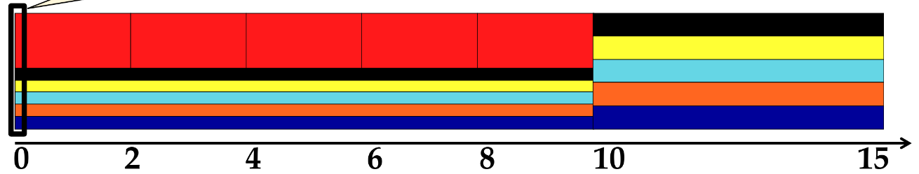
We construct an algorithm known as Weighted Fair Queuing on top of the GPS model. In essence, we utilize weighted round robin (WRR), in which the quantum of each task corresponds to its weight! This successfully approximates GPS—every period of $\sum_{i}w_{i}$ units of time, the processor will have done the same work as GPS. What WFQ is doing, essentially, is just choosing the task that finishes first in GPS within each time period, provided no other tasks are added to the system.

This following visualization of GPS may help show this dynamic of a task finishing first. Note that, here, the red task has a weight of 5, while the others have weights of 1.

Virtual Times

If other tasks are added into the system, the finishing times of each task may change! But, critically, the order in which tasks finish never changes (excluding the newly added task, of course, since it can be arbitrarily short/long). Thus, rather than scheduling tasks according to the physical finishing time, we track the number of WRR rounds needed to finish the task. This is known as the virtual finishing time. In essence, virtual time measures the service needed to complete a task. Note also that the system virtual time is thus the index of the round in the WRR scheduler.

More formally, let $V(t)$ denote the system virtual time. Then, the slope of $V(t)$, when graphed against $t$, represents the "normalized rate at which every task receives service in the fluid flow system." Naturally, the rate of $V(t)$ scales inversely proportional to the sum of the weights of all these tasks. In particular, $\frac{\mathrm{d} V }{\mathrm{d} t }=\frac{1}{\sum_{i}w_{i}}$. Note that $\sum_{i}w_{i}$ is equivalent to 1 virtual time unit. Then, in the ideal situation, for every time unit, each task should run exactly once (as it would in WRR).

In other words, as more tasks enter the system, the virtual time slows down!! Therefore, while every task's virtual finishing time stays the same, the virtual time progresses more slowly for each time quantum. In other words, $\frac{\mathrm{d} V }{\mathrm{d} t }$ decreases.

We can also calculate the virtual time from $0$ to $t_{1}$ as tasks are added/removed from the system. Just solving the differential equation above for $V$ provides

Since tasks enter/exit the system at discrete times, we can split this integral up into multiple integrals, with a new one each time the set of tasks changes (i.e. one per interval where the set of tasks is constant).

EEVDF

Earliest Eligible Virtual Deadline First is an algorithm that builds on top of these stated ideas. Like EDF, it schedules the task with the earliest deadline. However, unlike EDF, it uses virtual deadlines instead of physical deadlines, and only considers tasks that are currently eligible, where eligibility is calculated from a task's previously served requests.

Virtual time is essentially a representation of time weighted by the threads' weights. An increment of $t$ in real time corresponds to an increase of $\frac{t}{\sum w_{i}}$ in virtual time. In essence, you can think of it as a weighted average of all threads' progress. Then, if request $r$ from thread $i$ takes $t$ real time to complete, it should expect to complete it by within a duration of $\frac{t}{w_{i}}$, if provided its fair share.

More formally, we can write several recurrence relations that define the parameters of EEVDF.

• Recall that $S_{i}(t_{0},t_{1})$ denotes the virtual service time of a thread $i$ from $t_{0}$ to $t_{1}$.
• Let $t_{0}^{i}$ denote the time of the 1st request made by thread $i$.
• Let $ve(k)$ denote the virtual eligible time of the $k$th request.
• Let $vd(k)$ denote the virtual deadline of the $k$th request.
• Let $r(k)$ denote the request length of the $k$th request. This represents the ideal (with regards to fairness), real service time the thread should receive for this request between the virtual eligible time and virtual deadline, i.e. $r(k)=S_{i}(ve(k),\ vd(k))$.
• Let $w_{i}$ denote the weight assigned to thread $i$.

Then, we can write the following recurrence relations/equations.

Let's proceed through this step-by-step.

(1) First, the virtual eligible time of the first request is defined as the $V(t_{0}^{i})$, which is essentially the virtual time at which this thread makes its first request.

(2) The virtual deadline of the $k$th request is defined as the sum of the virtual eligible deadline and the virtual service time. Threads with a heavier weight will be assigned an earlier virtual deadline, since $\frac{r(k)}{w_{i}}$ will be smaller. In other words, threads with a higher priority will expect to finish sooner. Note that dividing $r(k)$ by $w_{i}$ essentially converts it to virtual service time!!

(3) The virtual eligible time of the $k+1$th request is equivalent to the virtual deadline of the $k$th request. The updates for the $k+1$th request only occur when the $k$th request finishes! This may take longer than one quantum.

The above is also very important to understand for the fairness of the theoretical/ideal EEVDF. Consider a request that finishes—its next virtual eligible time is updated to its previous virtual deadline, which represents the virtual time it should finish at in the idealized model of a fluid flow system. However, even if it finishes earlier than this, it should not be scheduled until after its previous, fair virtual deadline has been reached! This may be difficult to understand, so let's consider an example situation. There are two threads, each with equal weights of $1$ and requests of length $1$. They enter the system at the same time. Then, both start with an eligible time of $0$ and a deadline of $1$. As aforementioned, it's not possible to have generalized processor sharing on a processor; thus, one of these threads must finish first. Let's say we schedule thread $1$ first; it will finish its first request at virtual time $0.5$. Then, its new virtual eligible time will be updated to $1$. Why? Because it has already used up its fair time share in the time slice/quantum $0-1$. Therefore, it should not be scheduled again until virtual time has reached at least $1$, when it would be fair to schedule it again.

In a real-world CPU scheduling algorithm, step 3 changes slightly because lag can occur, since we do not know a priori how long a task will run for. Every time a quantum $q$ elapses, we compute $ve(k+1)=ve(k)+\frac{u(k)}{w_{i}}$, where $u(k)$ is the actual real service time that the request received. Note how, if $u(k)>r(k)$, the eligible time of this request gets pushed back more than it would have originally been. This is because the request received more time than it should have, i.e. negative lag, and thus its unfairly receiving more time. Similarly, if $u(k)<r(k)$, the eligible time of this request gets pushed back less than intended. This is compensating for positive lag, and ensuring this request gets scheduled sooner since it didn't receive as much time as expected.

Fun Fact!
EEVDF was introduced to replace CFS as the default scheduler in Linux kernel version 6.6.

Aside: Linux $O(1)$ Scheduler

This scheduler was used in the Linux kernel until version 2.6.

Note that the Linux $O(1)$ scheduler is a priority-based scheduler, with nice values of $[0,100)$ reserved for the kernel and $[100,140)$ reserved for the user. A lower nice value means a higher priority, and vice versa. The priority of each task determines its timeslice, like an MLFQ. Notably, there are also two separate task queues: an active and expired queue. Tasks that use up their timeslice are placed in the expired queue; once the active queue is empty, the queues swap.

The scheduler also leverages several $O(1)$ heuristics, including:

• User task nice value adjusted $\pm5$ based on p->sleep_avg = sleep_time - run_time. A higher sleep average corresponds to a more I/O bound task, and are provided higher priorities (lower nice values).
• Interactive credit: $+1$ when a task sleeps for a long time, $-1$ when a task runs for a long time. Tasks with high interactive credit may be placed back on the ready queue. Note that it can be negative! It's used to avoid impacting the responsiveness of interactive tasks by understanding one-off behaviors of tasks. This is important in the following scenarios:
  • Low interactivity task enters uninterruptible sleep; p->sleep_avg is high after exiting sleep. However, it's not actually interactive; it should not be prioritized by the scheduler. With interactive credit, it will have spent enough beforehand such that this one long sleep will not impact its interactive credit much $\implies$ scheduler knows this is a task that runs for a long time on processor (i.e. is not interactive).
  • High interactivity task uses up a lot of CPU time once. Again, its high interactive credit means it will not be penalized for high CPU usage once.
• Real-time tasks
  • Always preempt non-RT tasks
  • No dynamic priority adjustment
  • FIFO or RR (among same priority tasks)

Aside: CFS

The Completely Fair Scheduler is a scheduling algorithm designed to split CPU time between runnable tasks as fairly as possible. It was introduced in Linux kernel version 2.6, and phased out in version 6.6. Essentially, it keeps track of the virtual time of each task, ordered in a red-black tree. Then, it simply chooses to run the task with the smallest virtual runtime, i.e. the task that has received the least execution time so far. Note how CFS essentially replaces the previous $O(1)$ heuristics (except for RT tasks), as tasks that sleep more will naturally be scheduled sooner.

However, we don't just want fairness in the Linux scheduler. We want to prioritize low latency and starvation freedom too.

• Constraint 1: Target Latency
  • i.e., period of time over which every process is guaranteed service at some point
  • $\text{Quanta}=\frac{\text{Target Latency}}{n}$
  • However, if $n$ is too large, the time slice becomes too large, and context switching overhead becomes significant! This is reminiscent of the problem with RR. This impacts throughput negatively.
• Constraint 2: Minimum Granularity
  • i.e., minimum length of any time slice
  • Ensures context switching overhead never outweighs the time slice.

Nice values still exist in Linux, though—how does CFS account for this?

The answer is changing the rate of CPU cycles given to threads. Consider two threads $A$ and $B$, where $A$ has weight $4\times$ that of $B$. Then, while the virtual CPU time of both tasks in the red-black tree will be the same, the physical CPU time of $A$ will be $4\times$ that of $B$'s. (i.e., the virtual CPU time of $A$ advances $4\times$ slower than $B$'s). In fact, this is precisely the notion of weighted virtual time seen in EEVDF!